Evaluating the analytical performance of direct-to-consumer gut microbiome testing services

Experimental design strategy

As part of its mission to promote U.S. innovation and industrial competitiveness, NIST has been working with stakeholders in industry, academia, and other government agencies to develop standards to support the advancement and commercial translation of microbiome science. To this end, we wished to assess the current state-of-the-art with respect to DTC gut microbiome testing services. To achieve this, we deployed a NIST-developed human gut microbiome (human fecal) standard to assess the precision/reproducibility of seven DTC gut microbiome testing companies. For each of the seven companies, three tests/kits were ordered via the company’s website. Upon receipt of the (3 × 7 = 21) sample collection kits, we used a homogenized pool of human fecal material to serve as the test sample material for each collection kit. Collection procedures were followed according to instructions provided by each company (Table 1). Samples were placed into the company-provided shipping container and returned to the company for analysis. Results, in the form of company-specific reports, were received anywhere from 2 to 8 weeks following shipment of the sample. Taxonomic profiles were manually extracted from these reports and used for all subsequent analyses. It is also noteworthy that the companies were not informed of the ongoing assessment until after all the samples had been processed and final reports were received by NIST. Full details on materials and methods can be found in the Methods section.

Methodological parameters varied between companies

The process of translating the composition of stool sample into a microbiome report is multifaceted. As there are currently no universally accepted best practices for these methods, each provider likely employs a unique and often proprietary workflow. Microbiome measurements are impacted by a vast number of methodological variables including (1) sample collection, storage, and shipping methods, (2) nucleic acid extraction techniques, (3) NGS-library preparation, (4) sequencing technology, and (5) bioinformatic analyses. Bias can be introduced at every step, and even minor changes in methodology can lead to significant differences in results. In this study we had limited knowledge of the workflows that were employed by each company; however, we were able to infer key differences in both sample collection and sequencing methodologies.

Table 1 shows a comparison between companies regarding some methodological variables likely to impact the result (Table 1). Notably, there was considerable variability in methods for sample collection, including both the sample type (whole bowel movement vs. used toilet paper) and the sampling implement. Furthermore, some companies instructed users to add the sampling implement to a buffer, or to resuspend the sample in a buffer and discard the implement, while others directed users to ship the implement back ‘neat’, enclosed in a secondary sterile container. None of the shipping packages included ice, so all samples were shipped under ambient conditions (the study was conducted in the spring). The exact transit times between shipping and receipt of samples were not reported by all companies. Typically, notification of sample receipt or processing was sent 5 days – 7 days after shipping.

Regarding sequencing methodologies, some companies used marker gene amplicon sequencing while others relied on WMS. Among those using amplicon sequencing, one utilized 16S rRNA gene amplicon sequencing of the V3-4 region and the other two used 16S rRNA gene amplicon sequencing of the V4 region; additionally, one company included sequencing of internal transcribed spacer (ITS) amplicon for fungal identification. The read length and depth of sequencing, which can impact the specificity and sensitivity of taxonomic identification, varied by company. Although a wide range of read depths were reported, the variability within a single company was generally narrower (Table 1). Read depth ranged from <2 × 10⁴ to >1 × 10⁷. Interestingly, higher read depths did not always correlate with a greater number of species identified. For example, the three replicates from company C each reported over 600 species with read depths between 2 × 10⁴ and 3 × 10⁴. In contrast, company D reported 95, 98, 99 species for their three replicates, each with read depths exceeding 1 × 10⁷ reads. Although most details of read processing were not disclosed, we noted different cutoffs (ranging from 0.1% to 8 × 10⁻⁶ %) for reporting taxonomic assignment based on the taxonomic tables provided.

Taxonomic profiles varied across companies

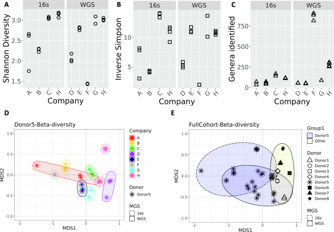
The process of generating the taxonomic tables from the data provided by each company required manual curation, as the reports came in varied formats (e.g., PDF, HTML). Additionally, a complete taxonomic profile was not part of Company A’s report but was obtained after sending a request to their help center. For comparison, NIST (referred to as company H) also performed metagenomic analyses on aliquots of the same material (donor 5) that was shared with the DTC companies. In addition, taxonomic data from 7 other unique donors (donors 1, 2, 3, 4, 6, 7, 8) were included in the NIST workflow to enable a comparison of the differences associated with biological variability (donor) vs. technical (methodological) variability. Although species-levels taxa were reported by each DTC company, all subsequent analyses at NIST were conducted using genus-level taxa assignments. A comparison of alpha diversity revealed a range of diversity values with no clear patterns based on read depth or sequencing method (Fig. 1A–C, respectively). Bray-Curtis dissimilarity was calculated to compare all replicates from each of the seven companies and NIST (company H) (Fig. 1D). Along with the alpha-diversity plots, the ordination plot can indicate inter-lab reproducibility. Tighter distribution of points in scatter plots (Fig. 1A–C) and on the ordination plot (Fig. 1D) suggest higher reproducibility for a company (e.g., Company F), while Company A showed poor reproducibility. Moreover, there was no distinctive clustering based on whether WMS or amplicon sequencing was used (WMS shown with solid lined, and 16S rRNA gene amplicon sequencing with dashed lined ellipses in Fig. 1D). One question raised was how the diversity observed for a single sample analyzed by multiple companies compared to biological diversity from different donors analyzed by a single workflow. A second Bray-Curtis dissimilarity index was calculated that included data from seven additional donors processed with the NIST workflow. Surprisingly, the diversity observed for samples from a single donor analyzed by different companies (asterisk in Fig. 1E, blue ellipses) appeared to be greater than or equal to that of biologically distinct samples (Fig. 1E, other shapes, yellow ellipse). This demonstrates that methodological variability can be greater than biological variability.

While Fig. 1E provides a visual representation of this variability, we also sought a more quantitative way to compare the methodological (between companies) and biological (between donors) variability. Figure 2, show a ratio of methodological to biological variance; a complete description of this analysis is available in the “Methods” section. Briefly, a Bayesian approach was used to determine the variation resulting from different methods being applied to the same samples (company analysis of Donor 5) and the variation resulting from a single method applied to multiple donors (NIST analysis of all 8 donors). This approach was applied to only the common taxa for this demonstration. The scatter cloud displayed in the figure represents 100 draws per sample. The sampling is reproducible (seed set), and we verified that subsampling does not materially alter the posterior summary statistics. Crucially, the full posterior summary (posterior mean and 95% credible intervals shown in red, blue, and black) is overlaid and remains the basis for inference. As shown in Fig. 2, only one genus (Haemophilus, shown in black) had a mean value and interval completely below 1, indicating there was less variation between methods than between donors for this genus. In contrast, 17 of the 18 taxa either had an interval completely above 1 (methodological variability exceeds donor) or had an interval that crossed 1 (similar variability between method and donor). This figure further supports the conclusion that methodological variability can be of the same magnitude as biological variability, and for some genera, methodological variability exceeded that observed between donors. Additionally, this figure reiterates that bias is often taxa-specific, an observation that is masked when summary metrics such as β-diversity and ordination plots are used.

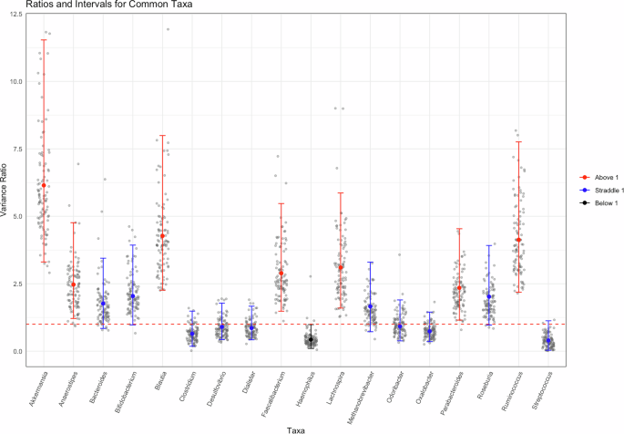
For the 18 genera that were identified in at least 1 replicate by each company, we fit a Bayesian hierarchical model. The ratio of the two variance components (colored, solid points) and the 95% credible interval surrounding (error bars) it are plotted. To visually represent posterior uncertainty without overwhelming the figure, gray points represent a randomly subsampled 100 draws per taxon, displayed in the scatter-cloud. This ensures a representative spread of the posterior while preserving figure clarity. The red, dashed line designates 1 on the graph. An interval fully above 1 (red) indicates that the methodological variability is greater than biological variability with 95% confidence; an interval that straddles 1 (blue) indicates that there is no significant different between the two variance components with 95% confidence; and an interval that is fully below 1 (black) indicates that the methodological variability is less than the biological variability with 95% confidence.

In addition to comparing diversity metrics, the taxonomic composition was compared on a genus-by-genus basis to identify the genera common to all analyses. For this analysis, any taxa that was not given a specific genus designation was renamed unspecified, and these assignments were then grouped with any unidentified taxa that were noted in the report. While some companies provided information that allowed us to determine the percentage of unidentified reads, this was not true across all companies. In fact, the NIST analysis, based on Bracken, removed unidentified reads prior to calculating relative abundance. Therefore, while we were able to show this data for some companies, absence of the unspecified category in Fig. 3 does not indicate 100% of the taxa were identified but could indicate that the unidentified reads were dropped earlier in the process, prior to calculating relative abundance values for known taxa. Despite vast differences in read depths, it was hypothesized that the most common genera would be present in all samples, and less abundant genera would only be seen in samples with higher coverage. The number of identified genera ranged from 34 to 906, with a relatively narrow range for each single company (Fig. 1C). From all 9 analyses (7 companies and NIST WMS and 16S rRNA gene amplicon sequencing), a total of 1208 unique taxa were identified. Only 3 genera were found in all samples when comparing all taxonomic profiles (Supplementary Fig. 1). A single replicate from Company A had a distinctive taxonomic profile (Fig. 3B, and observed in Fig. 1D as the single red asterisk on the left), which when removed from the analysis, increased the number of common genera to 17. This accounted for less than 2% of the total genera identified, or between 2% and 43% for any given sample. In most cases, these common genera constitute a majority of the genera (>50% of the abundance for companies A, C, D, G, and both NIST analyses), or the majority of genus-level specified reads (companies B and F). Additionally, the conservation of identified genera between replicates varied, from as low as 6% for Company A to as high as 98%. Excluding Company A, the genera conserved between replicates from the same company accounted for at least 95% of the identified sample composition. This indicates that most variability between replicates from a single company occurs among taxa present at low abundance and highlights the importance of empirically determined read cut-offs for taxa inclusion in a report.

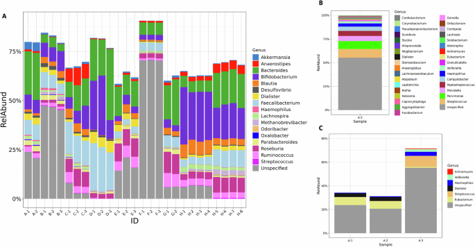
A The relative abundance of genera that were identified in all but one test. Each company is indicated by a letter, with replicate samples indicated by the number after the dash. B Relative abundance data for the one test sample (A-3) that was excluded from the overall analysis. All genera that were identified are included in the plot, C Relative abundance of genera found in common across replicates run by company A. The gray portion in all bars represents taxa that were not given a Genus level identification; this includes both taxa designated at a higher taxonomic level or that were listed as unidentified.

Replicate 1 from Company A had a significantly different taxonomic profile compared to the two other replicates from Company A and those from other companies (Fig. 3B). This egregious anomaly prompted further investigation. Compared to replicates 1 and 2 from Company A, replicate 3 had approximately half the number of reads (186 k compared to just over 400 k). This might have contributed to its distinct profile, as only 6 genera were common between replicate 3 and replicates 1 and 2, corresponding to 10% of the total genera and abundance for these replicates. In contrast, replicates 1 and 2 shared 69 out of 70 and 71 genera, respectively. Notably, the other 28 genera in replicate 3 were not unique but were identified in at least one other replicate across all the companies. It is also worth noting that the percentage of unspecified reads in replicate 3 comprised over 50% of the sample, whereas the unspecified designation accounted for just over 20% in replicates 1 and 2. These discrepancies raise concerns not just because the profile was distinct from other replicates originating from the same sample, but also because it apparently passed all quality control checks from the company, resulting in a report being generated and sent back to the customer.

Figure 3 provides a qualitative comparison of the relative abundances for different common taxa reported by each company. To quantify the level of agreement between companies, we examined the results on a taxa-by-taxa basis using a Bayesian approach that’s common in interlaboratory studies. The same 18 genera from Fig. 2 were analyzed, and the consensus value (Fig. 4 and Supplementary Fig. 2, yellow horizontal line) and corresponding uncertainty (Fig. 4 and Supplementary Fig. 2, shaded yellow region) from all nine measurements (7 companies and 2 methods from NIST) were determined. Depending on the genera being evaluated a range of comparability was observed (Fig. 4, Supplementary Fig. 2). Of note, no method reported concordance with the consensus relative abundance range for all 18 taxa analyzed. Rather, for any given method, the number of taxa where the relative abundance overlapped with the consensus range ranged from 10 to 16 taxa. In general, companies observed a genera dependent difference for outliers, reporting higher relative abundances for some and lower for others. Company A and H were the exceptions. Two genera (Blautia and Roseburia) from Company A had values outside of the consensus range, and the relative abundance for both genera was lower than the consensus ranges. For Company H, regardless of sequencing method (16S or WMS), when relative abundance values were outside of the consensus range, they were higher than the consensus range. From a genera specific perspective, Streptococcus was the only genera where the relative abundances for all 9 methods overlapped with the consensus range. Roseburia had the least agreement with only 3 of the 9 methods reporting relative abundance values that overlapped the consensus range. Whether measurement variability was greater than or indeterminate from biological variability (Fig. 2) did not appear to be a predictor of agreement for a given genus. An average of 2.9 outliers were observed for genera where methodological variability was greater than biological (Supplementary Fig. 2), and an average of 3.1 outliers were observed for genera where biological and methodological variability were indistinguishable (Fig. 4). It’s important to note, that these results are not indicative of accuracy since we do not know the actual composition of these samples. Instead, this analysis shows the agreement (or lack thereof) between companies (methods) for a given taxa and provides a means to quantify the level of that agreement.

Hierarchical Bayesian random effects model with a dark uncertainty was determined to compare individual company findings (A-G) and NIST findings (H₁-WGS, H₂-16S) to a consensus value (shown by yellow line), range (shown by yellow shaded region) for the 10 genera in Fig. 2 with variance ratios that straddle 1. The O’s indicate the average value for each company using 16S analysis and the X’s indicate the average value for companies using WMS. Thick gray lines represent the variability for each company, and the thin gray extensions capture additional variability attributed as dark uncertainty (further explained in the “Method” section).

Health indicators differ across companies

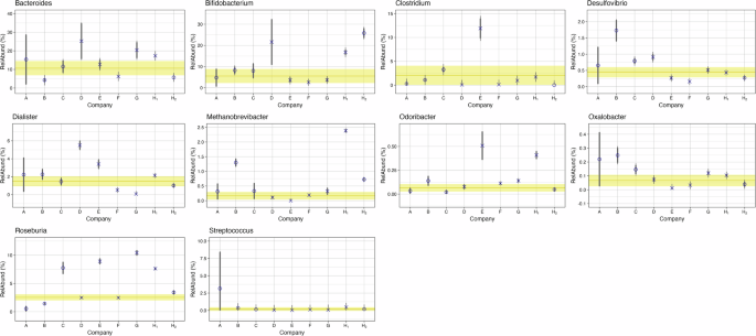
In addition to providing customers with a taxonomic profile, many reports also include health metrics, such as comparing a customer’s specific taxonomic profile to that of a comparator group. Notably, the comparator group varies between companies. For instance, Company E uses an internally developed dataset from a “healthy” cohort, while other companies rely on external datasets, such as those from the Human Microbiome Project¹⁶ or American Gut⁹. Beyond providing comparative data, some companies also identify beneficial or harmful microbes and suggest ways to modulate these microbes’ abundance to improve health. To examine how results vary between companies on a taxa-by-taxa basis, five clinically relevant genera were selected (Fig. 5 (A) Bacteroides (B) Bifidobacterium (C) Clostridium (to include Clostridioides) (D) Faecalibacterium and (E) Roseburia). All results were compared to the criteria provided by two of the companies. One company reported average values of the 5 genera in their reference population (Fig. 5, gray dotted line), and the other company reported an interquartile range (IQR) of their reference population (Fig. 5, range between the 25% and 75% bounds shaded in yellow). Interestingly, except for Bifidobacterium, the average used by one company does not fall within the IQR used by the other company. Variability between companies is observed for all five genera, with no apparent correlation to library preparation (16S rRNA gene amplicon sequencing vs WMS). In addition, the precision from a single company varied based on taxa, with some taxa showing indistinguishable points between replicates (e.g., Fig. 5E, Roseburia for companies D and F) and others showing wide variability (Fig. 5B, Bifidobacterium for company D). The implications of this variability are particularly evident in the health recommendations commonly included in DTC microbiome testing reports. The most striking example is of the conflicting recommendations between replicate 3 from Company A and replicates 1 and 2. For instance, starch breakdown was assessed as a metric for gut health; replicate 3 scored below average, whereas replicates 1 and 2 scored above. Out of the 10 functional categories assessed by this company, seven were below average for replicate 3, compared to only one for replicates 1 and 2, and the below-average category for replicates 1 and 2 was distinct from the seven observed for replicate 3. The company reported the microbiome as healthy for replicate 1 and 2, but unhealthy for replicate 3, which could lead to unnecessary interventions if such a report was received by a consumer. While Company A provides an extreme example, other discrepancies, including the identification of pathogens, were observed between different companies. For example, all of the companies evaluated (excluding NIST which restricted analysis to the genus level) provided information on Clostridioides difficile; however, of the seven companies, three indicate C. difficile was present and the other four reported absence.

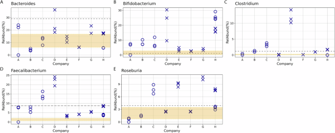
Relative abundance for select genera A Bacteroides B Bifidobacterium C Clostridium (to include Clostridioides) D Faecalibacterium and E Roseburia were plotted compared to reported comparators from company G as a gray dashed line and from company E as a shaded yellow region. The gray dashed line represents the average from the American Gut Project reported by company G as a comparator. The yellow shaded region indicates the IQR used to define the healthy population as a comparator used by company E. The symbols indicated metagenomic analysis: X’s designate companies using 16S amplicon sequencing and O’s designate WMS analysis. Three replicates are shown for each Company except for Company G which only had 2 successful samples and company H for which 4 samples were analyzed by both 16S and WMS resulting in 8 data points.