Cell-free chromatin state tracing reveals disease origin and therapy responses

by isenews 5 March 2026 0 Comment

Patients

The research presented in this study complies with all the relevant ethical regulations at their respective centres. Informed consent was obtained from all individuals or their legal guardians before blood sampling. Blood samples of patients with CRC were collected from Shanghai Tongren Hospital Hongqiao International Institute of Medicine and Ruijin Hospital affiliated to the Shanghai Jiao Tong University Medical School. Blood samples of patients with DLBCL, MCL, FL, tFL, TCL or CHD were collected from Peking University Third Hospital. Blood samples of self-claimed healthy individuals were collected and screened from Peking University Third Hospital and Chinese PLA General Hospital. Blood samples of patients with IBD were collected from Peking University first hospital and Ruijin Hospital affiliated to the Shanghai Jiao Tong University Medical School (Supplementary Table 6). This study was approved by the Ethics Committee of Peking University Third Hospital (S2024679), Ruijin Hospital (S2020384), Renji Hospital (KY2020-180), Chinese PLA General Hospital (S2023-806-01) and Peking University first hospital (S2021-389-001).

Clinical variables

Histological subtypes of each cancer type (DLBCL, MCL and FL) profiled in this study were established according to clinical guidelines using microscopy and immunohistochemistry and served as ground truths for assessing classification performance by trained pathologists. Cell-of-origin subtypes of DLBCL were assessed based on the Hans classifier per World Health Organization (WHO) guidelines⁶⁵. For B cell lymphoma and DLBCL subtypes profiled in previous studies by RNA-seq, we relied on subtype labels from their respective resources. tFL samples were obtained during the period of morphologic transformation from FL to DLBCL. The transformation was validated through immunohistochemical staining or fluorescence in situ hybridization testing. All lymphoma specimens were re-reviewed and classified according to the WHO classification⁶⁶. Samples of tFL were excluded from other analyses, except for the transformation analyses in Fig. 5, owing to their unique characteristics as an intermediate stage with high heterogeneities⁶⁷. Totally, 15 samples from 6 patients with tFL were used in the analysis. Notably, three patients (tFL-1, tFL-2 and tFL-5) underwent longitudinal sampling at various time points throughout the transformation period. CRC, CRA, CHD, IBD and B cell lymphoma samples were from patients in both pre-treatment and in-treatment phases. The primary treatment strategies for patients diagnosed with DLBCL, MCL and FL were R-CHOP-like therapy, R-CHOP/R-DHAP alternating therapy and R/G-CHOP therapy (Supplementary Table 7). Specifically, the in-treatment patients with DLBCL included in our study received a variety of treatment regimens, tailored according to the individual clinical context and response to prior therapies. The majority of patients were treated with standard first-line chemotherapy regimens, such as R-CHOP or R-CHOP-like treatment. Treatment response was evaluated after two cycles of treatment according to Lugano 2014 criteria.

The extranodal involvement sites in patients with B cell lymphoma were determined by PET–CT. Organ involvement sites and metabolic tumour volume in patients with cancer were also determined by CT and PET–CT. Colorectal precancerous lesion in patients with CRA was diagnosed by colonoscopy. True primary diseased tissues and cells in each group of patients were determined according to their primary clinical diagnoses (for example, lymphocytes were determined as the primary diseased tissues or cells in patients with lymphoma). True affected tissues and cells in patients with CRC were determined as organ involvement sites and metastatic organs. True affected tissues and cells in patients with lymphoma were determined as the extranodal involvement sites. Other clinical indices were mostly collected by clinical blood test. Progression-free survival and overall survival were calculated from time of treatment initiation. Overall survival events were death from any cause; progression-free survival events were progression or relapse, unplanned retreatment and death resulting from any cause.

Barcoded Tn5 preparation

The procedure of Tn5 expression, purification and assembly was followed as previously described^68,69,70,71. In short, pTXB1-Tn5 was transformed into BL21 (DE3)-competent cells and colonies were selected in 500 ml lysogeny broth (LB) medium and cultured at 37 °C overnight. Tn5 expression was induced by adding 0.2 mM isopropyl-β-d-thiogalactoside when the optical density of the bacteria culture reached 0.5–0.8 and bacteria culture was incubated at 23 °C, 80 rpm for 5 h. Bacterial pellets were collected and lysed by HEGX (20 mM of HEPES at pH 7.2, 0.8 M of NaCl, 1 mM of EDTA, 0.2% Triton X-100 and 10% glycerol) buffer with proteinase inhibitors cOmplete (Roche 04693132001). Bacteria were lysed by brief sonication. Genomic DNA in the lysate was precipitated by addition of polyethyleneimine (Sigma P3143) and clear lysate was incubated with 5 ml chitin rosin (NEB S6651L) at 4 °C for 1 h with rotation. The lysate–chitin rosin mix was loaded into a 10 ml column and washed with HEGX buffer. Following this, HEGX buffer containing 100 mM DTT and Roche cOmplete proteinase inhibitor was added to the column and incubated at 4 °C for 36 h. The eluted Tn5 protein solution was dialysed against 2× dialysis buffer (100 mM HEPES at pH 7.2, 0.2 M NaCl, 0.2 mM EDTA, 2 mM DTT, 0.2% Triton X-100, 20% glycerol), and then concentrated by centrifugation.

Assembly of Tn5 transposome was described previously^68,70,72. In brief, all oligonucleotides (Supplementary Table 2) were dissolved in TE buffer (5 mM Tris pH 8.0, 5 mM NaCl, 0.25 mM EDTA) to make 200 μM stock solution. To anneal adapters, each T5 or T7 oligos were mixed with equal volume of MErev oligo, placed at a thermal cycler for 5 min at 95 °C followed by programmed temperature decrease at 0.1 °C s⁻¹ to 75 °C, and left in 75 °C water to naturally cool down to room temperature. The 37.5 μM barcoded Tn5 transposome complex was obtained by adding 37.5 μM annealed adapters, 37.5 μM transposase Tn5 and storage buffer (50 mM HEPES pH7.2, 100 mM NaCl, 0.1 mM EDTA, 1 mM DTT, 0.1% Triton X-100, 60% glycerol) and incubating at 25 °C for 60 min. The assembled Tn5 transposome was stable and could be stored −20 °C for at least half a year.

Plasma sample collection

Blood samples were collected in K2 EDTA tubes, transferred to ice and added proteinase inhibitors cOmplete (Roche 04693132001) and 10 mM sodium butyrate (Sigma) within 4 h. The blood was centrifuged (1,500g, 10 min, 4 °C) to remove blood cells. Supernatant was transferred to a new tube and centrifuged again (3,000g, 10 min, 4 °C). The supernatant plasma was used freshly or flash frozen and stored at −80 °C.

Spike-in chromatin preparation

It is important to note that chromatin was used in two distinct contexts for entirely different purposes in this study. First, each plasma sample in 96-well plates was spiked with a constant amount of S2 chromatin to serve as a technical control (spike-in control, the analytic pipelines can be found in Supplementary Note). Second, in a separate application, varying amounts of S2 cells (original commercial source: Thermofisher, R69007) or CRC tumour-derived chromatin were added to assess the sensitivity of cf-EpiTracing in detecting external chromatin apart from human healthy plasma. Cell line identity was assessed based on characteristic morphology and growth properties, and all cell lines tested negative for mycoplasma contamination.

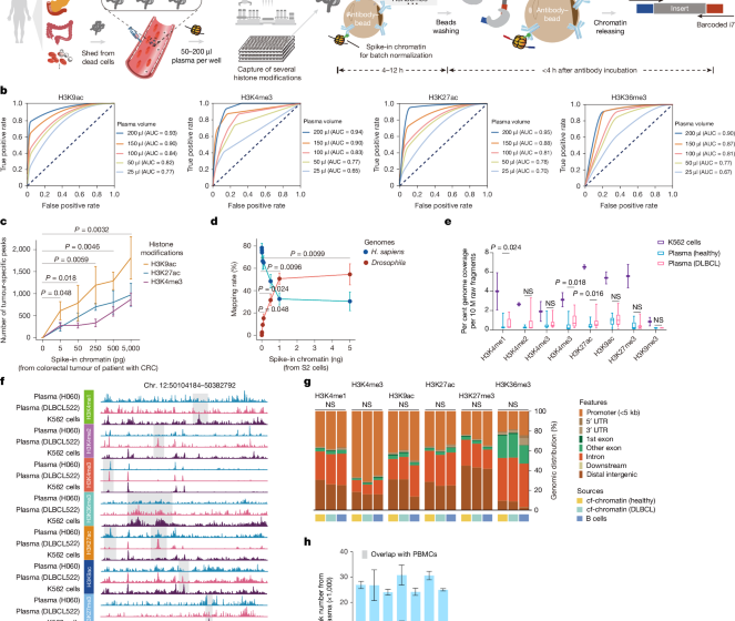
Spike-in S2 chromatin for normalization were prepared as previously described by sonication^36,73,74,75. In brief, 1 million fixed S2 cells (fixed in 1% FA on ice for 5 min) were resuspended in 500 µl hypotonic buffer (0.3% SDS, 20 mM HEPES, pH 7.9, 10 mM KCl, 10% glycerol, 0.2% NP-40) by pipetting and incubated on ice for 20 min. Pellets were collected by centrifugation at 3,000g for 5 min, then resuspended in 30 μl of nuclei lysis buffer (1% SDS, 10 mM EDTA, 50 mM Tris-HCl, pH 8.0), and lysed at 4 °C for 30 min. The sample was mixed with 70 μl of dilution buffer (0.01% SDS, 1% Triton X-100, 2 mM EDTA, 20 mM Tris-HCl pH 8.0, 200 mM NaCl) and transferred to 200 μl PCR tube. Chromatin was sheared into fragments of about 300 bp with a Qsonica Q800R2 sonicator. After centrifugation at 20,000g for 15 min, the supernatant was subpackaged and stored at −80 °C, which could be directly used in cf-EpiTracing. The DNA representation in the sonicated chromatin was quantified after phenol-chloroform extraction using Qubit. Specifically, the sonicated S2 chromatin, derived from approximately 3,000 S2 cells (equivalent to about 1 ng of DNA), was spiked into each well containing 200 µl human plasma. Native cfDNA is estimated to be present at approximately 1 to 5 ng in 200 µl of plasma. Consequently, the estimated ratio of spike-ins (sonicated fixed S2 chromatin) to native cfDNA in plasma would be approximately 0.2 to 1.

Spike-in CRC tumour chromatin and S2 nucleosomes for sensitivity analyses were prepared as previously described by MNase digestion. In brief, cells were resuspended in 200 μl nuclei extraction buffer (20 mM HEPES pH 7.5, 150 mM NaCl, 2 mM EDTA, 0.5 mM spermidine, 0.05% digitonin, 0.01% NP-40, 1× protease inhibitors, and 2% BSA) and incubated for 3 min on ice to extract nuclei⁷⁶. Nuclei were then centrifuged at 600g for 3 min and resuspended in 20 μl nuclei lysis buffer. The sample was mixed with 20 μl of MNase reaction buffer (2× Micrococcal Nuclease Buffer, 2 mM DTT, 4 U μl⁻¹ MNase). Reaction was activated at 37 °C for 5 min. 8 µl stopping buffer (50 mM EDTA, 0.5% Triton X-100, 0.5% DOC) were added and the reaction was incubated on ice for at least 15 min to stop the MNase digestion. Digested nucleosomes were subpackaged and stored at −80 °C.

cf-EpiTracing experimental procedure

Antibodies were conjugated to magnetic beads (Invitrogen 14301) according to the manufacturer’s instruction, including anti-H3K4me1 (Diagenode C15410194), anti-H3K4me2 (Diagenode C15410035), anti-H3K4me3 (Diagenode C15200152), anti-H3K27ac (Abcam ab4729), anti-H3K9ac (Active Motif 91103), anti-H3K36me3 (Active Motif 91265), anti-H3K27me3 (Cell Signaling 9733S) and anti-H3K9me3 (Abcam ab8898). Conjugated antibody–beads were stored in antibody storage buffer (0.05% sodium azide in PBS) at 4 °C.

Approximately 0.05 mg antibody–beads (with about 1 µg antibody), proteinase inhibitors cOmplete, 10 mM sodium butyrate and S2 chromatin were added into 200 µl plasma. Rotating the mixture overnight at 4 °C allowed capturing of cf-chromatin on antibody–beads. Beads were magnetized and washed three times with cold wash buffer (50 mM Tris-HCl, pH 7.4, 150 mM NaCl, 0.5% Triton X-100, 2 mM EDTA, 10 mM sodium butyrate) and once with 10 mM Tris-HCl, pH 7.4. Antibody–beads were then resuspended in 10 µl tagmentation buffer (10 mM MgCl₂, 10 mM TAPS-NaOH, pH 8.5, 100 nM Tn5 with barcodes). Reaction was activated at 37 °C for 30 min. Two microlitres of lysis buffer (60 mM Tris-HCl, pH 8.0, 60 mM EDTA, 0.25% SDS, 0.6 mg ml⁻¹ Proteinase K (Qiagen)) were added and the reaction was incubated at 55 °C for 15 min to stop tagmentation and digest proteins. Five microlitres of quench buffer (60 mM MgCl₂, 0.36% Triton X-100, 4 mM PMSF) was added and incubated at 37 °C for 15 min.

To each well, 30 µl PCR mix (10 µl 5× KAPA High GC enhancer buffer, 1.5 µl 10 mM dNTP Mix, 1 µl 25 mM MgCl₂, 0.5 µl 1U µl⁻¹ KAPA HiFi DNA polymerase, 17 µl H₂O) and 1.5 µl 10 mM i5 index primer and 1.5 µl 10 mM i7 index primer were added (Supplementary Table 2). PCR enrichment was performed in a thermal cycler: 1 cycle of 72 °C for 5 min; 1 cycle of 95 °C for 3 min; 21 cycles of 98 °C for 20 s, 65 °C for 30 s, 72 °C for 1 min; 1 cycle of 72 °C for 5 min, hold at 4 °C. Product was purified by 1.2× AMPure XP beads (Beckmann) twice and now ready for sequencing. The libraries were sequenced with paired-end 150-bp reads on the DNBSEQ-T7 platform.

To adapt to automated platforms, we optimized several steps of cf-EpiTracing experiments. In brief, we increased the volume of tagmentation buffer and lysis buffer to reduce DNA loss during automated operation. We also optimized running parameters such as prewetting tips, tip touching in dispensing, dispensing speed and dispensing height from the bottom of the tube. To avoid bubbles during liquid transfer, we disabled air blowout parameter in aspiration, and slowed down aspiration speed. The silicone soft cover, PCR plate, and matching ring-shaped magnetic stand were used in the automated pipeline. In addition, we used two heating oscillators alternately to control the temperature and reduce waiting time.

In situ ChIP with tumour tissues

In situ ChIP was performed as previously described⁷⁰. Tissues were crushed into pieces with an automated homogenizer (IKA), washed twice with PBS to remove blood, and then resuspended in 100 µl antibody buffer (20 mM HEPES pH 7.5, 150 mM NaCl, 0.5 mM Spermidine, 1× cOmplete inhibitor (Roche), 10 mM sodium butyrate, 0.07% Triton X-100, 0.01% Digitonin, 2 mM EDTA). Antibodies (anti-H3K4me3, Diagenode, C15200152, 1:100 dilution; anti-H3K9ac, Active Motif, 91103, 1:100 dilution; anti-H3K27ac, Abcam, ab4729, 1:100 dilution) were added to each group of tissue and incubated at 4 °C overnight. Tissues were washed twice with washing buffer (20 mM HEPES pH 7.5, 150 mM NaCl, 0.5 mM spermidine, 10 mM sodium butyrate) with 0.01% digitonin. Samples were resuspended in 100 µl antibody buffer with secondary antibodies (Donkey anti-rabbit-Alexa 488 (1:500 dilution; Invitrogen, A32790) and Donkey anti-mouse-Alexa 555 (1:500 dilution, Invitrogen, A31570)), and incubated at 4 °C for 30 min, followed by washing twice with wash buffer with 0.01% Digitonin. Finally, samples were suspended with 100 µl washing buffer with 0.07% Triton X-100 and 0.01% Digitonin, 1× cOmplete inhibitor, and 3 µg ml⁻¹ PAT-MEAB. The tissue pieces were incubated at 4 °C for 1 h and washed with 180 µl washing buffer with 0.01% Digitonin and 0.05% Triton X-100. Reaction was activated by suspending samples with 50 µl reaction buffer (10 mM MgCl₂, 10 mM TAPS-NaOH, pH 8.5, 1× cOmplete, 10 mM sodium butyrate), followed by gently flicking and incubated at 25 °C for 1 h in a PCR cycler. To stop the reaction, 40 µl 40 mM EDTA was added, followed by further incubation at room temperature for 15 min. Samples were washed twice with 0.1% BSA/PBS. Samples were finally resuspended with 20 µl lysis buffer (10 mM Tris-HCl, pH 8.0, 0.05% SDS and 0.1 mg ml⁻¹ Proteinase K), and incubated at 55 °C for 10 h, then 85 °C for 30 min to deactivate Proteinase K. Four microlitres of 1.8% Triton X-100 was added and incubated at 37 °C for 30 min to quench SDS.

Five microlitres of tissue lysates of each sample was divided into a new tube. To each well, 42 µl PCR mix (10 µl 5× KAPA High GC enhancer buffer, 1.5 µl 10 mM dNTP Mix, 1 µl 25 mM MgCl₂, 0.5 µl 1U µl⁻¹ KAPA HiFi DNA polymerase, 19 µl H2O) and 1.5 µl 10 mM Nextera index i5 primer and 1.5 µl 10 mM Nextera index i7 primer were added. PCR enrichment was performed in a thermal cycler: 1 cycle of 72 °C for 5 min; 1 cycle of 95 °C for 3 min; 16 cycles of 98 °C for 20 s, 65 °C for 30 s, 72 °C for 1 min; 1 cycle of 72 °C for 5 min, hold at 4 °C. Product was purified by 1× AMPure XP beads. Size selection was carried out by first 0.5× AMPure beads to remove >1 kb fragments, and second 0.5× AMPure beads to the supernatant to obtain 200–1,000 bp fragments. The libraries were sequenced with paired-end 150-bp reads on the DNBSEQ-T7 platform.

Mapping, visualization, peak calling, correlation and heat maps

We filtered out sequencing reads by indexing barcode sequences with any mismatch. After removing adapters and low-quality bases by cutadapt (v.1.11), paired-end cf-EpiTracing reads were mapped to the human reference genome hg19 and Drosophila reference genome dm3 using Bowtie2 (v.2.2.9)⁷⁷. Uniquely mapped reads with map quality greater than 30 were used for the following analyses, using Samtools (v.1.9). PCR duplicates were removed by Picard (v.2.2.4) (http://broadinstitute.github.io/picard). Only uniquely mapped, non-duplicated reads were used for analysis. To visualize cf-EpiTracing signals, we used Deeptools BamCoverage (v.3.5.1)⁷⁸ to normalize and calculate coverage in continuous 50-bp bins in bam files and generated track files (bigwig format). cf-EpiTracing signals were visualized in track view using Integrative Genomics Viewer (v.2.3.59)⁷⁹. Heat maps and average curves were generated using Deeptools (v.3.5.1). Peaks were identified using MACS2 (v.2.1.1)⁸⁰ with the parameter setting (–nolambda –nomodel –broad) with different cut-offs for different histone markers. Peaks with distance within 1,000 bp were merged for further analysis. Genomic correlations were calculated using normalized average signals in either genomic windows, transcription start site (TSS) regions or peak regions by multiBigwigSummary function in Deeptools.

Receiver operating characteristic curve for accuracy

We assessed the quality of cf-EpiTracing data generated from 25–200 µl of plasma by constructing ROC curves (as shown in Fig. 1b), and conducted benchmarking analyses between cfChIP and cf-EpiTracing (as shown in Extended Data Fig. 2b). Sensitivity analyses focused on the peak regions of H3K4me3, H3K9ac, H3K27ac and H3K36me3 signals, which were used as the primary regions for subsequent analyses. The benchmarking analyses concentrated on the peak regions of H3K4me1, H3K4me2, H3K4me3 and H3K36me3 signals, which were also characterized in previous cfChIP analyses¹⁰. In each histone modification comparison, comparable sample sizes were used. cf-EpiTracing was performed with 200 µl of plasma, and cfChIP was performed with approximately 2 ml of plasma, using either cf-EpiTracing or cfChIP profiles as gold standard.

We focused on signal peaks on promoter regions (defined as 10,000 bp upstream and 10,000 bp downstream of a TSS for H3K4me1, H3K4me2, H3K4me3, H3K9ac and H3K27ac, and gene body regions in the hg19 genome for H3K36me3). The gold standard true positives were defined as the set of high-confidence peaks on either promoter regions or gene body regions identified in merged data. The set of promoter regions that did not overlap with any peaks was defined as the gold standard negative set. Using the gold standard sets, the following quantities were defined to compute the ROC curve: true positives (TPs), peaks that were supported by the gold standard positive set; false positives (FPs), peaks that were not supported by the gold standard positive set; false negatives (FNs), gold standard positives that were not called peaks in an experiment; true negatives (TNs), peaks that were not called in an experiment and were in the gold standard negative set. True positive rate (TPR) was defined as TP/(TP + FN) and false positive rate (FPR) was defined as FP/ (FP + TN). ROC curves were generated by computing TPR and FPR values on prediction sets obtained by varying the peak-calling threshold, as described in previous studies^81,82.

Integrated analysis of multiple histone modifications

To capture the significant combinatorial interaction between different histone modifications in their spatial context (ICSs) across collected epigenomes, we used ChromHMM (v.1.23)^41,83, which was based on a multivariate hidden Markov model. A ChromHMM model applicable to all collected epigenomes of tissues and primary cells was learned by virtually concatenating consolidated data corresponding to the core set of seven chromatin marks (H3K4me1, H3K4me3, H3K9ac, H3K9me3, H3K27ac, H3K27me3 and H3K36me3) assayed in all reference epigenomes (Supplementary Table 4). For each consolidated ChIP–seq dataset, read counts were computed in non-overlapping 200-bp bins across the entire genome. Each bin was discretized into two levels, 1 indicating enrichment and 0 indicating no enrichment. We decided to use an 18-state model for all further analyses as they retained all the key interactions between these chromatin states. The trained model was then used to compute the posterior probability of each state for each genomic bin in epigenome of both plasma samples and reference (tissues and primary cells). For each epigenome, chromatin states were labelled in 200-bp resolution using the state with the maximum posterior probability on corresponding regions.

Definition of tissue-specific sites with ICSs

To define tissue-specific sites of ICSs, we examined the specificity of every genomic 200-bp bins. For each site, we judged whether it was tissue-specific of certain chromatin states by examining whether they were exclusively labelled in one tissue or primary cell. Specifically, tissue-specific regions were defined by the criteria that the posterior probability on corresponding regions were higher than 0.9 in only 1 tissue or primary cell and lower than 0.1 in other tissues and primary cells. For example, region A was labelled as ICS 1 (ICS13) in tissue C, which was unique in tissue C among all tissues and primary cells. In this case, region A was the tissue-specific region of tissue C in ICS13. For each tissue or cell type, there were various tissue-specific genomic regions defined by 18 ICSs. To this end, we obtained tissue-specific sites (tissue signatures) of all 65 tissues or cells in 18 ICSs.

Calculation of signals of tissue signatures for plasma samples

We first used bed format files containing genomic distribution regions of selected histone modifications (H3K4me3, H3K9ac and H3K27ac) for defining genome-wide ICSs. Genomic regions were discretized into two levels, 1 indicating enrichment and 0 indicating no enrichment, using the BinarizeBed function of chromHMM. Binary files were next input into 18 chromatin states as described above and genomic annotation was performed in 200-bp resolution, using MakeSegmentation function of ChromHMM and makewindows function of bedtools (v.2.30.0)⁸⁴. In each ICS, we searched for events that cf-chromatin from plasma captured tissue-specific signals. For example, region A was annotated with ICS 13 in tissue C, which was unique in tissue C compared to other tissues and cell types. Region A was the tissue-specific region of tissue C in ICS13. The detection of ICS13 labelling in this genomic region in plasma samples was defined as the event of capturing tissue-specific signals in tissue-signatures. ICS13 of tissue C. We summarized the counts of such events across 18 ICSs, resulting in a vector containing 1,170 values (tissue–signatures.ICSs, 65 tissues or cell types multiplied by 18 ICSs). This matrix represents the captured events in tissue-specific regions across the 65 tissues and primary cells for 18 ICSs. The scores in this vector are referred to as signals for tissue signatures.

Unsupervised clustering analyses

We performed unsupervised clustering analyses to compare the contribution of each histone modification in accurately clustering tissue/primary cell samples (from bulk ChIP–seq data) and plasma samples (cf-EpiTracing data from patients with DLBCL and healthy controls). For tissue and cell clustering, signals from genomic regions representing tissue-specific ICSs across 65 tissues or cells were computed using combined histone modification data derived from ChIP–seq datasets. For plasma sample clustering, signals corresponding to ICSs specific to B cells (54 tissue-signature ICSs from CD19-positive cells, naive B cells and GCBs) were calculated using combined histone modification data from cf-EpiTracing of plasma samples. To assess the minimal requirements for clustering performance, each of the six histone modifications was respectively excluded from the integrated analysis to evaluate its individual importance.

For each histone modification combination, signals in tissue-specific ICSs, comprising samples from 10 distinct tissue types (with 5 replicates per type in tissue and cell clustering analyses) or 2 distinct plasma sample groups (n = 15 for healthy individuals and n = 15 for patients with DLBCL in plasma clustering analyses), were first transformed and normalized using Seurat (v.4.3.0). log-normalization with a scale factor of 100,000 was applied, followed by the identification of highly variable features using variance-stabilizing transformation. PCA was then performed to reduce the dimensionality of the data and facilitate visualization based on these variable features.

To evaluate clustering accuracy, k-means clustering was applied. In tissues and cell types clustering analyses, samples were partitioned into ten clusters corresponding to the known tissue types. For plasma clustering, k-means partitioned the samples into two clusters, reflecting the known sample groups. Clustering performance was quantified using NMI and ARI, both calculated against the true sample labels, as described in previous studies^85,86,87.

A Pearson correlation matrix was generated based on signals from the variable features, and hierarchical clustering was conducted using Euclidean distance. The resulting correlation heat map enabled visual assessment of sample similarity and clustering accuracy. Hierarchical clustering results were further evaluated using NMI and ARI to assess their consistency with the known tissue/plasma classifications.

Identification of differential ICSs

To identify the differential ICSs among different groups of individuals (for example, CRC-specific ICSs compared with healthy individuals), bed format files of selected histone modifications (H3K4me3, H3K9ac and H3K27ac) were used in the definition of genomic ICSs. For group A (for example, patients with CRC) and group B individuals (for example, healthy individuals), genomic regions were first discretized into two levels, 1 indicating enrichment and 0 indicating no enrichment in 5,000-bp resolution. Binary files were next input into 18-state chromatin states as described above and genomic calculation of posterior probability of each ICS were conducted, using MakeSegmentation function of ChromHMM with the additional option “-printposterior”. We annotated genomic 5,000-bp regions with R package ChIPseeker (v.1.5.1)⁸⁸ based on human genome (hg19). We next preserved genomic regions that were annotated to cover the regions from upstream 20,000 bp of TSS to downstream 20,000 bp of TES genome-wide. These regions may jointly participate in gene regulation of corresponding genes. We summarized scores of 18 ICSs of certain genes by summing score from the same categories. In this way, 18 ICS scores were obtained for each gene, jointly reflecting their regulatory states. Differential analyses of ICS scores between groups of individuals were performed with the R package DESeq2 (v.1.44.0). In brief, a threshold of |log₂(fold change (FC))| = 1 and adjusted P value = 0.05 was applied in identification of differential ICSs, using the Benjamini–Yekutieli procedure to control for false discoveries.

Selection of ICSs in downstream diagnostic and prognostic analyses

The 18-ICS ChromHMM model was trained using all eight histone modifications from tissue and primary cell samples. This model leverages state transition probabilities to accurately infer chromatin states, even when using a subset of histone modifications⁴¹. We determined that the combination of H3K4me3, H3K9ac and H3K27ac, associated with regulatory elements such as promoters and enhancers, was of paramount importance in defining the 18 ICSs. Therefore, subsequent cf-EpiTracing analyses focused primarily on these histone modifications.

Based on the emission probabilities for chromatin state definition and the transition possibilities between chromatin states, ICS1, ICS2, ICS3, ICS4, ICS5, ICS8, ICS10 and ICS11, which were predominantly associated with heterochromatin and gene bodies, were difficult to distinguish from one another using a combination of signals from H3K4me3, H3K9ac and H3K27ac (Extended Data Fig. 3b,c). Consequently, we prioritized the selection of the 10 most relevant ICSs (ICS6, ICS7, ICS9, ICS12, ICS13, ICS14, ICS15, ICS16, ICS17 and ICS18) that could be clearly distinguished using these histone modifications for downstream analyses including diagnostic and prognostic biomarker discovery, unbiased disease screening, patient stratification and subtyping, as well as machine-learning-based classification models.

GLM analyses

To assess the distinguishability of tissue signature-associated ICS signals among patients with CRC, CHD or B cell lymphoma, GLMs were implemented. The entire dataset (n = 125 for healthy individuals, n = 107 for patients with CRC, n = 23 for patients with CHD and n = 309 for patients with B cell lymphoma) was randomly partitioned into two subsets for each classification task: 80% of the samples were allocated for model training, and the remaining 20% were reserved for independent model testing. Differential analyses of tissue-signature ICSs was conducted to identify disease-specific tissue-signatures for CRC, CHD and lymphoma, using 342 tissue-signature ICSs linked to the primary diseased tissues across the three disease categories. The selection process involved comparing each disease group against all other samples in the training dataset.

Separate GLMs were constructed for CRC, CHD and lymphoma using a binomial logistic regression framework, incorporating the respective disease-specific ICS signatures identified from the training dataset. Model parameters were estimated via maximum likelihood estimation, optimizing the log-likelihood function to minimize classification error.

Model performance was assessed using the independent testing dataset, which was strictly withheld from both feature selection and model training phases. Area under the receiver operating characteristic curve was computed to evaluate classification effectiveness.

Development of unbiased screening model

An unbiased screening model was predicated on the assumption that primary diseased tissues and affected or involved tissues increased tissue-specific signals due to elevated levels of excessive cell death and replenishment. This leads to an overrepresentation of tissue-derived signals in patients compared to healthy individuals. For each tissue or cell type, we assigned diseased condition when the signal exceeded a threshold defined by healthy individuals. This method is designed to detect not only cancer-related changes derived from tumour tissues but is also applicable to various other diseases with tissue lesions.

To determine these thresholds, we statistically assessed the distribution of signals from all tissue-signature ICSs (n = 1,170) in healthy individuals using the descdist and fitdist functions in the R package fitdistrplus (v.1.1-11). Our analysis showed that the signals in tissue-signatures ICSs follow a normal distribution in healthy population. A normal distribution was then fitted for each of the 1,170 tissue-signatures ICSs in healthy individuals, with the 90th percentile (upper quantile) used as the threshold to differentiate between outlier and control profiles. For each tissue-signatures ICS, the signal was discretized into two categories: ‘1’, indicating a disease signal (when the signal exceeded the 90th percentile threshold) and ‘0’, indicating a control signal (when the signal was below this threshold).

The tissue enrichment score for each tissue was calculated by summing the disease signals and divided by the total number of selected tissue-signature ICSs for that tissue. Each type of tissue or primary cell is characterized by ten tissue-signatures.ICSs (in ICS6, ICS7, ICS9, ICS12, ICS13, ICS14, ICS15, ICS16, ICS17 and ICS18). Given that some tissues often exhibited concurrent lesions in disease states, we aggregated tissue-signatures.ICSs for these tissues in the calculation of enrichment scores into broader categories. For example, the enrichment score for the colorectum was calculated on the aggregated tissue-signatures.ICSs of colonic mucosa, colon smooth muscle, rectal smooth muscle, rectal mucosa and large intestine. Similarly, heart enrichment scores were generated by combining scores from the right atrium, right ventricle and left ventricle; lymphocyte enrichment scores were calculated from CD19-positive cells, GCBs and naive B cells.

To enhance the detection of signals in diseased tissues, we used random forest-based feature selection to identify tissue-signatures.ICSs that most effectively distinguish patients and healthy controls. Random forest is well-suited for this task as it ranks features by importance without extensive parameter tuning and has been widely used in feature selection. We ran the random frorest algorithm 10 times, each with 100 trees, and used the mean decrease in Gini impurity to assess feature importance. Importance scores from each run were averaged to minimize variance and obtain stable feature rankings. Top 5 features (tissue-signatures.ICSs) with the highest average importance scores were selected to be used in calculating tissue enrichment for each tissue. By narrowing down tissue specific ICSs that contributed most to the differentiation between patient and control groups, we enhanced the ability of our model to distinguish between patients and healthy controls. This scoring enabled screening of 65 tissues and primary cells.

The identification of primary diseased tissues was based on the combined tissue enrichment scores from all categories, with the highest score corresponding to the tissue with the highest likelihood of being diseased. Affected or involved tissues were defined as those tissue categories of elevated enrichment scores.

For example: if we screen liver-specific tissue-signatures.ICSs in a tested sample and find that 3 out of 5 selected liver-specific tissue-signatures.ICSs exceed the 90th percentile threshold defined in healthy individuals. The liver enrichment score in this case is 3/5 = 0.6. Among the enrichment scores for all tissues, the liver shows the highest score, suggesting that the liver may be the primary diseased tissue for this sample.

Detection of tumour-derived signals in plasma

Tumour-derived ICSs of each patient with CRC was identified by performing comparative analyses using ChIP–seq data of tumour (this study) and normal tissues from healthy donors (public data). We defined cancer-specific sites as |log₂(FC)| > 1 between ICS scores in tumours and normal tissues. Also, we removed sites in which sums of ICS score in patients with CRC and healthy individuals were lower than 0.5. Notably, the primary diseased tissues of patients with CRC were mainly nominated as colon and rectum. Cancer-specific ICSs in tumours were defined by comparing with both normal colon (colonic mucosa and colon smooth muscle) and normal rectum (rectal smooth muscle and rectal mucosa).

Cancer-specific ICSs in plasma of each patient with CRC were identified by performing comparative analyses using cf-EpiTracing data of plasma from patients and healthy individuals. We defined cancer-specific sites as |log₂(FC)| > 1 between ICS scores in plasma from patients and healthy individuals. We removed sites, in which sums of ICS score in patients with CRC and healthy individuals were lower than 0.5.

Tumour-derived signals captured in patient plasma were defined as cancer-specific ICSs detected in both tumour and plasma of patients and healthy individuals. The significance of the overlap was evaluated by hypergeometric test with R function hyper. P value < 0.05 was determined as statistically significant. We used non-cancer controls and shuffled controls in the analyses to verify the high specificity of cf-EpiTracing in detecting tumour-derived signals.

XGBoost machine learning

XGBoost machine learning models were developed to: (1) classify patients with CRC and healthy individuals, and detect early colorectal precancerous lesions (CRA); and (2) diagnose and grade patients with DLBCL at different stages. For each application, the models were designed with clear separation of training and independent validation groups. The models were trained and tuned using only the data from the training group. To optimize model performance, Bayesian optimization was employed to fine-tune key hyperparameters, including max depth, learning rate (eta), gamma, subsample ratio, colsample bytree, min child weight, alpha, lambda and scale pos weight. The optimization process for classification models aimed to maximize the area under the receiver operating characteristic curve and was conducted using ten-fold cross-validation over multiple iterations. For the regression models, optimization aimed to minimize r.m.s.e. through similar cross-validation methods.

Following optimization, the final models were trained on the entire training set using the best hyperparameters as follows:

a.

CRC-Healthy classification model: max_depth=5, eta= 0.2394864, gamma= 3.821408, colsample_bytree=0.8249388, min_child_weight=3, subsample= 0.5704591, alpha= 0.554617, lambda= 1.593141, scale_pos_weight= 2.569478.
b.

DLBCL score regression model: max_depth=10, eta=0.3, gamma= 0.279328905137363, colsample_bytree=0.524896209484371, min_child_weight=1, subsample= 0.614474824865937, alpha=1.86492748212796, lambda=2.22044604925031e-16, scale_pos_weight=3.33254521566179.

The models and training codes have been made available at https://github.com/Helab-bioinformatics/cf-EpiTracing. Comprehensive evaluations for overfitting, bias, class imbalance, robustness and reliability were conducted for each model. Overfitting was assessed and controlled through comparison of training and validation accuracy across training iterations (learning curves) and using ten-fold cross-validation in parameter tuning. Bias and class imbalance were evaluated using confusion matrices, while robustness and reliability were measured by accuracy, precision, recall, F1 score and AUC (for classifier model) and mean absolute error, root mean square error (r.m.s.e., for regression model). Performance was assessed in an external validation cohort to further evaluate the reliability and generalizability of the models.

Of note, samples from the validation group were sourced from an independent medical centre and separate patient cohort. CRC samples (n = 75) from the training group were collected exclusively from the Shanghai Tongren Hospital, Hongqiao International Institute of Medicine, and the CRC samples in the validation cohort (n = 32) were obtained from Ruijin Hospital, affiliated with Shanghai Jiao Tong University School of Medicine. Healthy donor samples in the training group (n = 93) were collected from Peking University Third Hospital, with those in the validation group (n = 32) sourced from the Chinese PLA General Hospital. DLBCL samples in both the training (n = 133) and validation groups (n = 37) were obtained from Peking University Third Hospital, but from distinct patient cohorts.

To evaluate the generalization capability of the CRC-Healthy classifier, it was applied to adenoma samples (CRA), which were an unseen subset of precancerous data. Each CRA sample was classified as either CRC or healthy based on a 0.5 probability threshold. Samples with predicted probabilities ≥0.5 were considered correctly detected as CRA.

For the DLBCL score regression model, the expected DLBCL scores for healthy individuals and patients in stages I, II, III and IV were set to 0, 1, 2, 3 and 4, respectively. The Youden index was used to determine the optimal cut-offs for DLBCL scores in the classification of training group samples, and these cut-offs were subsequently applied to the validation group samples (Fig. 5k).

Stratification of prognosis of patients with CRC

Differential analyses identified 747 ICSs that were significantly upregulated in patients with CRC compared to healthy controls in the discovery dataset. Hierarchical clustering of the 747 ICSs was performed on the discovery dataset, which divided patients with CRC into two subgroups, CRC-1 and CRC-2, based on distinct ICS patterns. Unsupervised hierarchical clustering was applied to the validation dataset using the same ICS clusters derived from the discovery cohort. Patients were classified into CRC-1 and CRC-2 based on their ICS profiles, which reflected the clustering pattern observed in the discovery dataset. Kaplan–Meier survival analysis was conducted to compare recurrence-free survival between CRC-1 and CRC-2 subgroups in both the discovery and validation datasets. log-rank tests were used to assess the statistical significance of survival differences between the subgroups. Survminer package (v.0.4.6) and Survival packages (v.2.44-1.1) in R were used for survival analysis.

Disease subtyping analyses in patients with B cell lymphoma

Tissue signatures were quantified by summing the tissue-signatures.ICSs of CD34-positive cells, naive B cells and GCB cells in patients with DLBCL, MCL and FL, respectively. Multi-class receiver operating characteristic analysis was performed to evaluate the performance of classifying B cell lymphoma subtypes (Fig. 5c,d).

Differential analyses were performed across all patients with B cell lymphoma (n = 170 for DLBCL, n = 74 for MCL and n = 65 for FL) to identify ICSs that were exclusively enriched in each lymphoma subtype. A threshold of |log₂(FC)| ≥ 1 and an adjusted P value ≤ 0.05 was applied. Hierarchical clustering was subsequently performed on patients to identify three distinct patient clusters, compared with their clinical diagnoses, and assess the clustering’s accuracy (Extended Data Fig. 8a,c). The same analyses were conducted using bulk RNA-seq data from tumour tissues (GSE32018 (GPL6480); Extended Data Fig. 8b,c).

Hierarchical clustering of GCB DLBCL and patients with non-GCB DLBCL was performed using the detected signals in tissue-signature ICSs associated with CD34-positive cells and naive B cells. This unsupervised clustering identified two distinct patient clusters, which were subsequently assigned to either the GCB DLBCL or non-GCB DLBCL subtype based on the signals from GCB cell-dominant ICS and CD34-positive cell-dominant ICS clusters. The subtyping performance was then benchmarked against the Hans classification, which is the clinically recognized gold standard for DLBCL subtyping (Fig. 5e,f).

Differential analyses were performed on all patients with DLBCL with clearly documented clinical records confirming classification as either the GCB (n = 45) or non-GCB subtype (n = 73), to identify ICSs that were exclusively enriched in each DLBCL subtype, using the threshold of |log₂(FC)| ≥ 1 and an adjusted P value ≤ 0.05. These two distinct patient clusters by hierarchical clustering were compared to their clinical diagnoses to evaluate the clustering performance (Extended Data Fig. 8g,i). The same analyses were performed using bulk RNA-seq data from tumour tissues (GSE31312 (GPL570); Extended Data Fig. 8h,i).

Identification of recurrence-related ICSs for DLBCL

We initially performed differential analyses to identify ICSs that were significantly upregulated in patients with DLBCL compared to healthy controls within the discovery dataset. A total of 432 ICS candidates were identified using the threshold of |log₂(FC)| ≥ 1 and an adjusted P value ≤ 0.05 under Benjamini–Yekutieli correction for further investigation. Each candidate ICS was individually evaluated for its association with DLBCL recurrence using a multivariate Cox proportional hazards model, adjusted for five established clinical indices: clinical stage, age at initial diagnosis, lactate dehydrogenase (LDH) levels, β2-microglobulin (β2-MG) levels, and white blood cell (WBC) counts. These indices are routinely used in clinical practice for disease monitoring and were included as covariates to account for potential confounding effects. Hazard ratios (HRs) with 95% confidence intervals were estimated, and statistical significance was assessed using Wald log-likelihood tests. In total, 8 ICSs were identified as significantly associated with disease recurrence, with an adjusted P values less than 0.05 after multiple testing correction (Bonferroni method). To validate the predictive utility of these ICSs in an independent validation dataset, not used in candidate selection, was used exclusively for external validation. We defined the integrated ICS score as the weighted average of 8 recurrence-related ICSs, with weights corresponding to the log HR values from the discovery dataset, reflecting their relative contribution to prognosis prediction. Prior to obtaining integrated ICS scores, the proportional hazards assumption was verified for each Cox model. The optimal threshold of integrated ICS score for stratifying patients into high- and low-risk groups was determined using maximally selected rank statistics (surv_cutpoint function from the R package maxstat, v.0.7.26) in the discovery dataset. This threshold was subsequently applied to both the discovery and validation datasets for risk stratification.

Kaplan–Meier survival curves were generated to assess whether the individual recurrence-associated ICS and integrated ICS score effectively stratified patients with DLBCL into distinct prognostic groups. Log-rank tests were conducted to compare survival outcomes between high- and low-risk patients. In parallel, similar analyses were performed to evaluate the prognostic value of clinical indices. Specifically, the IPI level cut-off that best separated patients with different survival probabilities was identified within the discovery dataset and subsequently validated in the external validation dataset. IPI was selected as a representative clinical index because it integrates key factors such as age, clinical stage, Eastern Cooperative Oncology Group (ECOG) performance status, and LDH levels, providing a comprehensive assessment of factors that are critical for assessing clinical treatment response.

Pseudo-time analyses

We conducted pseudotime analysis using Monocle3 (v.1.2.9) to delineate sample trajectories based on signals in genomic regions for all 1,170 tissue-signatures.ICSs. Highly variable features (500) identified with the FindVariableGenes function of Seurat was used to estimate similarities between DLBCL, FL and tFL samples. We first clustered and projected the samples on to a low-dimensional space (uniform manifold approximation and projection (UMAP)) in Seurat object. Pseudotimes were calculated according to similarities in the tissue-of-origin signals to reflect sample relationships during transformation. Monocle3 then resolved the FL-DLBCL transformation trajectories and calculated the pseudotime for each sample as shown in Fig. 5g.

Transcription factor motif analysis

In Fig. 5i, we used genomic 200-bp bins that were annotated as active integrative chromatin states (ICS6, ICS7 and ICS9–18) in each tFL sample but annotated as repressive chromatin states (ICS1–5 and ICS8) in 80% FL samples for transcription factor motif discovery for each tFL sample. We used genomic 200-bp bins that were annotated as active integrative chromatin states (ICS6, ICS7 and ICS9–18) in 80% DLBCL samples but annotated as repressive chromatin states (ICS1–5 and ICS8) in 80% FL samples for transcription factor motif discovery for DLBCL. Transcription factor motif analysis was conducted using the HOMER (v.4.11) transcription factor motif discovery algorithm, and P values were adjusted for multiple testing using the Benjamini–Hochberg procedure to control for false discoveries.

Detection of t(11;14) translocation events

The fragment size of cfDNA library was mostly below 150 bp, which was shorter than the sequencing read with the sequencing strategy adopted in this study (PE150). Thus, we assumed that reads capturing translocation event should be one side aligned to chromosome 11 with the other side aligned to chromosome 14, and such reads in whole could not be aligned to the genome. To screen out fragments that met our criteria, for each read that could not be aligned to human genome, we aligned the head 20 bp and the tail 20 bp to hg19 genome, respectively and preserved reads whose one side aligned to chromosome 11 and the other side aligned to chromosome 14. To eliminate false positives, for each pre-selected read, we further surveyed the other reads corresponding to the same fragment to test whether opposite results could be obtained as a cross-validation. For example, we preserved fragment A, in which the head 20 bp of read 1 aligned to chromosome 11 and the tail 20 bp of read 1 aligned to chromosome 14 while the head 20 bp of read 2 aligned to chromosome 14 and the tail 20 bp aligned to chromosome 11. We also excluded fragments whose alignment to chromosome 11 located outside the potential candidate loci in t(11;14) translocation (chr. 11: 69,229,598-69,455,854)⁵⁵. Total translocation events were determined as sum of all events detected in all H3K4me3, H3K9ac and H3K27ac cf-EpiTracing data. Translocation scores were defined by the translocation events (read counts with detected translocation events) detected in plasma samples.

Identification of ageing-related ICSs

Ageing-related differential ICSs were subsets of differential ICSs between patients (in this study, patients with MCL) and all healthy individuals that showed the ageing-related pattern. Around these sites, the difference between healthy individuals and patients gradually attenuated in older healthy individuals. Ageing-related differential ICSs were statistically defined as those showing the significant correlation between ICSs score and age in healthy individuals (adj. P value < 0.05 and Pearson correlation > 0.5). P values were adjusted for multiple testing using the Benjamini–Hochberg to control for false discoveries.

GO term enrichment analysis

Differential ICSs were identified through DESeq2 by comparing between the experimental and control conditions. Genes related to the differential ICSs were included in Gene Ontology (GO) term enrichment analyses. GO term enrichment analysis was performed to assess the biological significance of these genes. We used the enrichGO function from the clusterProfiler⁸⁹ package (v.4.10.0) to determine the overrepresentation of Gene Ontology (GO) terms across Biological Process, Molecular Function and Cellular Component⁹⁰. The background gene set for this analysis included all genes related to ICSs tested in the DESeq2 analysis, ensuring a comprehensive and unbiased comparison of gene ontology terms. Enriched GO terms were identified using a hypergeometric test, and P values were adjusted for multiple testing using the Benjamini–Hochberg to control for false discoveries.

Statistical analysis

Details of statistical analysis were as indicated in the text and figure legends. Statistical tests were two-sided unless stated otherwise. Results were considered significant at a P value threshold of 0.05. Two-tailed P < 0.05 was considered statistically significant unless stated otherwise. Multiple testing correction was performed using the Bonferroni, Benjamini–Yekutieli, or Benjamini–Hochberg procedure, when appropriate. Groups were compared using log-rank tests in Kaplan–Meier plots. The Wald log-likelihood test was used in the Cox proportional hazards model to assess the statistical significance of covariates. Paired two-tailed Student’s t-test was performed between two groups when appropriate. The Kruskal–Wallis test was used to evaluate the difference between groups to test whether they followed the same distribution. The hypergeometric test was performed to test the overlap significance. The asymptotic one-sample Kolmogorov–Smirnov test was performed to test the null hypothesis that the observed data followed a theoretical distribution.

Custom R scripts and R packages were used to generate heat map, violin plot, ridge map, bar plot, line chart, and boxplot, and perform statistical analysis. Plots were generated with Python (v.3.9.7), R (v.3.6.1) and Rstudio (v.4.2.2), using ggplot2 (v.4.3.2), pheatmap (v.1.0.12), radarchart (v.0.7.5) and euler (v.6.1.1).

Reporting summary

Further information on research design is available in the Nature Portfolio Reporting Summary linked to this article.

First Appeared on
Source link