Limited thermal tolerance in tropical insects and its genomic signature

Study area

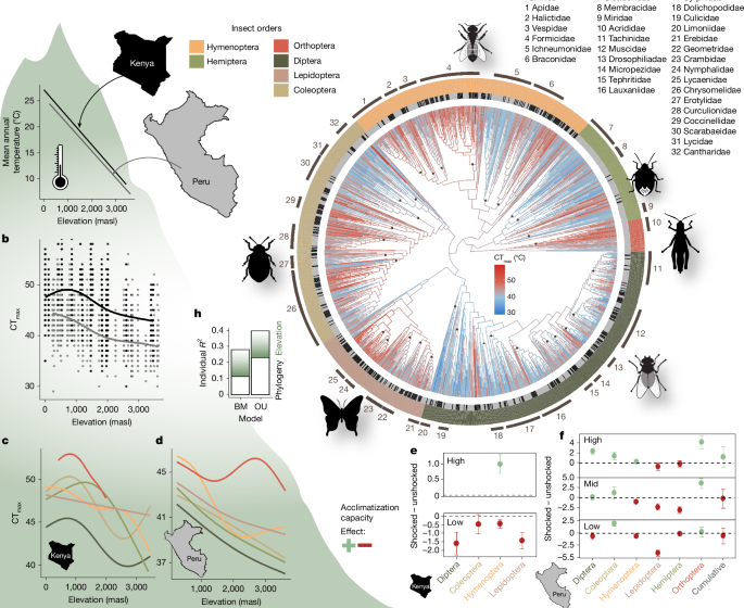
In Peru, the study was carried out along an elevational gradient from 245 masl to the tree line at 3,588 masl in the Andes of south-east Peru (Kosñipata valley), with continuous and mostly undisturbed wet rainforest/cloud forest. The climatic gradient has three seasonal periods with a wet season (November to March), a dry season (May to July) and austral spring (September and October)³⁹. Mean annual temperatures range from 24.3 °C in the lowlands to 6.7 °C at 3,600 masl (Fig. 1). Mean annual precipitation levels are high with >1,500 mm per year along the whole gradient, peaking at around 1,500 masl with ~5,000 mm (ref. ⁴⁰). Research was conducted on 26 study plots of approximately 100 m × 100 m in ~250 m elevation intervals and seven field stations distributed along the gradient. Four of the 26 plots were located inside Manú National Park. Nine of the plots matched the long-term research plots of the Andes Biodiversity and Ecosystem Research Group (ABERG) project⁴¹.

In Kenya, the study was carried out along an elevational gradient from 11 masl at Watamu to 3,450 masl at Mount Kenya including forests, woodland, scrub and grassland in natural and semi-natural habitats. The climate is mostly semi-arid in the lowlands to humid at higher elevations⁴² and characterized by seasonality in precipitation. Two rainy seasons occur from March to May and from October to December, a distinct season during the boreal summer from June to September, and a pronounced dry season in January and February^43,44. The forested parts of the Taita Hills region and Mount Kenya from ~1,300–2,500 masl are characterized by a tropical montane forest climate with generally high humidity and constant high precipitation (>1,500 mm). Mean annual temperatures range from 26.2 °C at the lowest plot to 8.9 °C at the highest plot (Fig. 1). In total, 15 study plots were selected in similar elevation intervals along the elevation gradient.

Insect collection

Insects of all major orders (mainly Coleoptera, Diptera, Hymenoptera and Lepidoptera; additionally, Hemiptera and Orthoptera) were collected in the Neotropics (n = 4,690) in three seasons (September to December 2022, April to August 2023, and September to December 2023) with sweep nets in the understory of all study plots. In the Afrotropics, insects (n = 3,164) were collected in one season (March to June 2023), applying the same method. We stored live insects in Eppendorf tubes with moist tissue and sugar solution, protected from the sun, and transported them back to the field station, where thermal tolerance measurements of all collected individuals were carried out on the same day. Insect collection was focused on taxonomic breadth covering six major orders rather than on individual species. Note, that our results represent the more common insect communities. In the Supplementary Methods, we provide extensive robustness analyses to assess the effects of incomplete sampling or modifications to the phylogeny.

Measuring thermal limits

We measured critical thermal limits (CT) by exposing the insects in individual plastic tubes (2, 5 or 50 ml, depending on body size) to decreasing (CT_min) or increasing (CT_max) temperatures using a programmable thermoblock (Eppendorf Thermostat C)^7,45,46. Each individual was only tested once. To avoid the effects of starvation, each tube was equipped with a piece of paper towel moistened with sugar water. For acclimatization to a common baseline, insects were first exposed to the starting temperature of 28 °C for 10 min. We then increased or decreased temperatures by 1 °C every 2 min—that is, a ramping rate of 0.5 °C min⁻¹—following standardized methods¹⁴. After each 2-min interval, we checked all insects for mobility. The temperature at the point of lost mobility, even after tapping or gently shaking the tube, was noted as the upper or lower thermal limit (CT_max or CT_min)^14,15. After the test, insects were stored in 96% ethanol for later genetic barcoding and specimen documentation. Since we did not directly measure the body temperature of the insects, CT_min and CT_max values determined with the above-mentioned protocol may not perfectly reflect body temperatures. Nevertheless, owing to the small size and their high surface-area-to-volume ratio, insects equilibrate to environmental temperatures quickly, typically within seconds⁶.

All thermal limit data were originally stored as csv or xlsx files (Microsoft Excel v.2502) and imported into R v.4.3⁴⁷. Since four different observers measured CTs in the field, we first tested for potential observer bias by evaluating the CT_max of lab-reared ants of one colony. Each observer measured CT_max of ten individual workers of the colony under the same conditions. We found no significant difference in mean CT_max across any of the observers (ANOVA, F_3,36 = 1.576, P = 0.212).

For investigating CT patterns along elevation gradients, we applied generalized additive models with elevation as a smooth term explanatory variable. We restricted the smooth term parameter k to 5 to avoid overfitting^48,49. Thermal tolerance ranges were calculated by subtracting mean CT_min from mean CT_max for each study plot. We checked the trend of thermal ranges along elevation with an ordinary linear model. We additionally applied the same models for each major insect order. Thermal safety margins were calculated for both datasets by subtracting plot-specific variables of mean annual temperature and mean daily maximum air temperature of the warmest month from the CT_max values. Both temperature data variables were derived from the CHELSA data base (bio1 and bio5 of the BIOCLIM+ dataset)⁵⁰.

As a test for plastic responses, a subset of insects was first exposed to heat (40 °C, n = 777 insects) or cold (14 °C, only in the neotropics, n = 490 insects) shock for 10 min prior testing, replacing the 28 °C acclimatization period. The sublethal temperatures for the heat shock were identified in pre-experiments. In the Neotropics up to an elevation of 2,700 masl, insects generally survived a 10 min shock of 40 °C; at higher elevations 35 °C was chosen as shock temperature, because a large proportion of the pilot test insects did not survive a 40 °C shock. After the shock, the standard protocol continued from 28 °C with temperature changes in 2-min intervals.

Plastic capacities were analysed by comparing CT measurements between individuals that were exposed or not exposed to a heat or cold shock before CT measurements. We added heat shock or cold shock (yes/no) as a variable for CT_max or CT_min, respectively, and calculated the means for both groups. Data were additionally grouped by elevation level (lowlands: <600 masl, mid: ≥600 masl and <1,200 masl, high ≥1,200 masl), because we expected heat shock effects to vary depending on elevation. We hypothesized that a thermal shock would increase tolerance—that is, have a positive effect. Therefore, for CT_max, effect calculations were done by subtracting the mean thermal tolerance of the control group from the mean thermal tolerance of the group exposed to a heat shock (‘shock yes’ – ‘shock no’). For CT_min, the calculation was done in reverse (‘shock no’ – ‘shock yes’), so that the effect direction remains the same, with a positive effect indicating an increased tolerance level.

Insect identification and phylogeny

All insects were morphologically sorted into orders and, where possible, families, and delimited into species-like units based on individual DNA barcoding. For this, we sampled tissue from all specimens that were tested for thermal tolerance and positioned them in a well filled with 30 μl of absolute ethanol (99.9%) in a 96-well microplate. Sequencing preparation and conduction was done at the Canadian Centre for DNA Barcoding (CCDB). Libraries were created for DNA barcoding (standard 658 bp COI (mitochondrial cytochrome c oxidase subunit I) barcoding) using SMRT sequencing technology on a PacBio Sequel IIe⁵¹. All genetic sequences were uploaded together with specimen photographs and sampling information to BOLD (database code DS-A2TP; https://www.boldsystems.org/). The COI sequences had an average length of 557 bp with a minimum overlap of 303 bp (74% of all COI sequences were larger than 500 bp and 50% larger than 600 bp).

We applied the BOLD sequence cluster tool which uses the refined single linkage (RESL) algorithm with a pairwise distance model to sort all insects into unique operational taxonomic units (OTU), which we used as species-like units (called ‘species’ in the text)⁵². Contaminants, records with stop codons and sequences with a length below 300 base pairs were excluded. In total, 4,300 barcoded individuals were included in the final phylogenetic analyses of which 2,330 were unique OTUs, resulting in an average of 1.8 individuals per OTU. The CT_max data included 2,246 measurements with 1.9 individuals per OTU, the CT_min data included 1,849 total observations with a mean of 2 individuals per OTU. We used the BOLD ID engine (minimum of 80% similarity to databased sequences) to allocate all sampled insects to family level⁵³.

We used R to create a phylogeny based on a family-level backbone tree and DNA sequences²⁰. For this, we downloaded an insect family-level backbone tree⁵⁴. For each family, a separate subtree was calculated first, using the AlignSeqs function from DECIPHER⁵⁵ and a maximum likelihood model (TreeLine function). Statistical support for each branch is provided by aBayes values (see data repository). If a family consisted of only one OTU, a ‘tree’ with a single branch of fixed length was constructed. Next, all subtrees were added to the ultrametric backbone tree using the bind.tree function from the ape package⁵⁶. Branch lengths were calibrated with the bladj function from phylocom⁵⁷, that estimates node ages based on fossil calibration points while unknown ages are evenly distributed between known nodes⁵⁴. For clearer visualization (Fig. 1h), terminal tip heights were equalized with the forceEqualTipHeights function from ips⁵⁸. Note that while this gives the appearance of an ultrametric tree, the branch lengths do not represent absolute time, but the result is a phylogeny with relative branch lengths. All scripts and details of phylogeny construction can be found in²⁰.

We reconstructed ancestral trait values of thermal tolerances using the fastAnc function from phytools⁵⁹, plotted them on the phylogenetic tree with ggtree⁶⁰, and calculated a phylogenetic correlogram using phylosignal to test for significance of the phylogenetic signal—that is, if trait values of related OTU are more similar (or dissimilar) than expected by chance²¹. The phylogenetic parameters Pagel’s lambda and Blomberg’s K were tested with the phylosig function and 10,000 randomizations. To disentangle the effects of adaptation or acclimatization to a local climate from those of phylogenetic relatedness, we applied a phylogenetic regression using the phylolm package, and function of the same name, with elevation as predictor and phylogenetic relationships entering a covariance matrix of the model either based on the assumption of a Brownian motion and an Ornstein–Uhlenbeck model of trait evolution⁶¹. We compare the Ornstein–Uhlenbeck and Brownian motion models since they represent two mechanistically contrasting hypotheses about trait evolution and are most commonly used in literature⁹. Under a Brownian motion model, traits are assumed to have evolved under random evolutionary drift, under an Ornstein–Uhlenbeck model with stabilizing selection towards an optimum. We calculated the evolutionary optimum for CT_max under an Ornstein–Uhlenbeck model—that is, the parameter θ, using the fitContinuous function of the geiger package⁶². We compared model performance using the Akaike information criterion⁶³. Variance partitioning to extract partial r² values was conducted on these models using the phylolm.hp package⁶⁴.

In order to verify the dependence of results concerning elevational trends in CT, on the reconstruction of ancestral traits, the estimation of a phylogenetic signal and of an upper boundary of CT_max (Ornstein–Uhlenbeck model), we conducted an extensive set of robustness analyses considering various modifications of the phylogenetic tree and various data subsets, which is described in the Supplementary Information, with results presented in Extended Data Fig. 3 and Supplementary Table 1.

Protein stability prediction

We predicted the thermal stability of proteins applying the deep learning model DeepSTABp²⁶. It uses a transformer-based protein language model to extract sequence embeddings, which are analysed with advanced deep learning techniques for large-scale protein stability predictions²⁶. To cover proteins from species across all insect orders, we downloaded all available genomes (protein format) from 677 insect species from InsectBase 2.0⁶⁵. This data covered 20 orders, 158 families and 457 genera. Next, in R, we imported all genomic data translated into amino acid FASTA files and then randomly selected 1,000 proteins per species, a trade-off to receive as many overlapping proteins between species as possible while keeping the following analyses at a feasible computation time. We set up a local version of DeepSTABp, to predict melting points for this large number of proteins. Anaconda PowerShell was used to create a conda environment and Python programming language (v.3.13) to run the script⁶⁶. In DeepSTABp, we set growth conditions to ‘cell’ and a default temperature of 22 °C (ref. ²⁶). For testing robustness of results, we conducted analyses with data from all genomes, only high-quality genomes (BUSCO > 89.9, N50 > 300 kb), and only for proteins which were covered by all insect species. Furthermore, for comparison we used data of all proteins and of the 25% proteins per species that showed the highest thermal sensitivity (n = 88,643 proteins from 677 species).

To investigate the underlying, structural mechanism of heat tolerance in insects, we predicted CT_max by protein melting temperatures T_m. Differences in T_m across orders and families were tested with mixed effect models (lme), setting species-specific protein identity as random term. For the comparison of T_m with field-measured CT_max, we calculated mean CT_max values for each family of the Afrotropical and Neotropical data. We calculated the 25% quantile of T_m for each species (that is, a proxy for an average T_m of temperature sensitive proteins) of the genomic dataset and then averaged these values among all species per family. Using a linear model (lm), we tested the relationship between T_m of the temperature sensitive proteins (average of the 25% quantile of T_m) and the mean CT_max of families. Here, we first calculated an unweighted linear model and, second, a model weighted for the number of species with genomic data in each family.

Climate data

On all Neotropical plots, one TMS-4 soil and one air temperature logger (TOMST) recorded air temperature at 15 cm and 2 cm above the ground, as well as soil temperature and moisture at −6 cm depth in 15-min intervals for approximately one year (September 2022 to December 2023)⁶⁷. Air temperature was additionally measured at 1.5 m height with iButton sensors (Analog Devices) in 240 min intervals. The sensors were protected from rain and sunlight using white plastic dishes (diameter 18 cm)⁶⁸. Air temperatures at 1.5 m (T_{air at 1.5 m}) were highly predictive of the temperature at 15 cm height (T_{air at 15 cm})—R² = 0.999, T_{air at 1.5 m} = 0.26673 + 0.99845 × T_{air at 15 cm}—and due to the denser sampling intervals, data of the TMS-4 sensor were used for final statistical analyses. At one plot (ID 056), the TMS logger could not be recovered due to fallen trees; therefore, the mean annual temperature from iButton data was used to predict T_{air at 15 cm} for this plot instead. For the East African study plots, we did not have temperature loggers available but retrieved comparable data by modelling shaded air temperatures using NicheMapR. We simulated hourly temperatures at every plot across one year (micro_global function). This climatic model takes detailed environmental variables into account, such as elevation, slope, solar radiation and absorptivity⁶⁹.

Additionally, for all study plots climate data (BIOCLIM+: mean annual air temperature (bio1); mean daily maximum air temperature of the warmest month (bio5); mean daily minimum air temperature of the coldest month (bio6)) were extracted from CHELSA data base. This dataset is based on temperature measurements of climate station from the years 1981–2010. This was done to have climate data with higher comparability between the geographic regions and to model future temperatures at the study plots. CHELSA was chosen as it is particularly suitable for modelling climate along mountain slopes due to its terrain-based downscaling of global data (https://chelsa-climate.org). Both bio1 and bio5 climatic variables were highly correlated to estimates of the same measures based on the field-measured climatic data (Extended Data Fig. 9 and Supplementary Information).

Surface temperatures for all study plots were derived from the ECOSTRESS sensor, a radiometer mounted on the International Space Station that measures surface temperatures with a resolution of 70 m (ref. ²⁹). As ECOSTRESS measures surface temperatures at a low temporal resolution and significant parts of the data were filtered due to low data quality (for example, due to cloud cover), surface temperature measurements of study plots were enriched by additional measurements of 50 randomly selected locations within a buffer of 5 km around each plot. For all additional locations the elevational level was determined using the NASA SRTMGL1 digital elevation model (v.003) with a spatial resolution of 1 arc-second (approximately 30 m). We applied a filter (binary ‘0b00’ = best quality retrieval) to only use high-quality surface temperature data. For better visualization, we only plotted temperatures above the 50th percentile of temperature values in Fig. 3.

Heat coma models

For better estimating the effects of current and future temperatures on tropical insects, we converted the dynamic CT values to static CT values and calculated heat coma times t_coma for present and predicted future environmental temperatures¹⁹. The static CT model includes a thermal sensitivity coefficient z, which describes how knockdown time changes with temperature. Across different insect species, z varies between 1 and 5, with an average value of 3 (ref. ¹⁹). To provide additional estimations of z, we tested ramping rates from 1 to 0.06 °C min⁻¹ with three species of leaf cutter ants in the Neotropics (Acromyrmex coronatus, Acromyrmex octospinosus and Atta colombica) as model organisms, since they could be easily found along an elevation gradient from 270–1,349 masl. In the ant data, we found z to range from 2.16–5.50 along the gradient, which overlapped with reports from the literature. For the final static value calculation, we used z = 3, following a conservative approach. Under the assumption of higher z values, t_coma would be shorter than the values reported in Fig. 3.

For the calculation of the effect of environmental temperatures on t_coma of insect communities under current climate and climate change scenarios we extracted community-level CT_max values from the lowest plot and applied it across the whole elevational gradient, a rather conservative approach, assuming that the thermal sensitivity of insects across the elevation gradient can, by species turnover, adaptation, or acclimatization, increase to values of CT_max currently found in lowland species. We calculated t_coma assuming an average CT_max (median CT_max of all lowland insects), for a 25% quartile of CT_max (termed ‘more heat-sensitive insects’) and for a 10% quantile of CT_max (‘most heat-sensitive insects’). In the Neotropics, the 10% quantile of all insects measured in the lowland CT_max was 40 °C, the 25% quantile was 41 °C, and the median was 42 °C. In the Afrotropics, the 10% quantile of CT_max was 43 °C, 45 °C (25% quantile) and 47 °C (median). For future climate projections (2071–2100) under the three shared socio-economic pathways SSP1-2.6 (sustainable scenario), SSP3-7.0 (medium-high scenario) and SSP5-8.5 (high scenario) we used the GFDL-ESM4 climate model predictions (highest priority; https://protocol.isimip.org/#/ISIMIP3b/biodiversity) of bio5 supplied by the CHELSA database⁵⁰. We extracted the mean daily maximum air temperature of the warmest month (bio5) and calculated the anomaly based on the difference between current and future bio5 temperatures (Extended Data Fig. 8). We then estimated the future air temperatures by adding these anomalies to the current environmental temperatures measured in the field (Neotropics) and modelled microclimate (Afrotropics), as well as for the surface temperatures (ECOSTRESS) on each plot. Using this approach, we incorporated the fine-scaled temporal variation in environmental temperatures along the Afrotropical and Neotropical elevation gradients to future climate projections. Thereby, we assume that the differences of environmental temperatures at small temporal scale to bio5 remains the same under future climate projections (details in Supplementary Information). We acknowledge that surface temperatures may not warm at the same rate than air temperatures. The difference between surface and air temperatures is expected to increase with increasing temperatures, particularly in open areas⁷⁰. Thus, our method provides conservative estimates of future surface temperatures. For calculating the percentage of critical temperatures (leading to heat coma within an exposure time of 8 h), we related for each study plot the number of critical temperatures to the total number of temperature values (including 100% of all temperature measurements—that is, including night temperatures).

While reported results are mainly based on the GFDL-ESM4 climate model, all analyses were additionally calculated with a multi-(climate) model ensemble. The detailed methods are described in the Supplementary Information and results of the multi-model-ensemble are shown in Supplementary Fig. 1.

Inclusion and ethics statement

Fieldwork in Peru and Kenya was conducted in collaboration with local research institutions, including the Universidad Peruana Cayetano Heredia and the Museo de Historia Natural in Lima, and the University of Embu in Kenya. All necessary permits were obtained from the respective national authorities (see Acknowledgements). Local scientists were involved in study design, data collection and manuscript preparation, and are included as co-authors. Field logistics were supported by local assistants, who are acknowledged accordingly. The research supported local capacity building through training initiatives and shared data access. The collection of biodiversity data addresses locally relevant priorities and contributes to future monitoring and conservation efforts.

Reporting summary

Further information on research design is available in the Nature Portfolio Reporting Summary linked to this article.