Multi-modal spatial characterization of tumor immune microenvironments identifies targetable inflammatory niches in diffuse large B cell lymphoma

Human research ethics approval

This study was approved by the Institutional Review Board of The University of Texas MD Anderson Cancer Center (protocol PA19-0420) using archival samples and a waiver of informed consent. The sex and age of study participants are provided in Supplementary Table 1. No compensation was provided to participants.

CosMx SMI assay

To obtain a quasi-3D transcriptomic dataset, formalin-fixed, paraffin-embedded (FFPE) tissue blocks were sectioned to 5 μm slices using a microtome. The sample processing, staining, imaging and cell segmentation were performed as previously described. In brief, tissue sections were placed on VWR Superfrost Plus Micro Slides (cat. no. 48311-703) for optimal adherence. Slides were then dried at 37 °C overnight, followed by deparaffinization, heat-induced antigen retrieval and proteinase-mediated permeabilization (https://nanostring.com/products/cosmx-spatial-molecular-imager/single-cell-imaging-overview). Then, 1 nM RNA-in situ hybridization probes were applied for hybridization at 37 °C overnight. After a stringent wash, a flow cell was assembled on top of the slide, and cyclic RNA readout on CosMx was performed (Human Universal Cell Characterization RNA 1K-plex panel). Before starting RNA detection cycling, morphology markers for visualization and cell segmentation were added, including pan-cytokeratin (PanCK), CD68, CD298/B2M, CD45 and DAPI. Over 40 FOVs (0.509 mm × 0.509 mm) were selected for data collection on each slice. The commercial CosMx optical system has an epifluorescent configuration based on a customized water objective (×22.7/1.1 NA) and uses widefield illumination, with a mix of lasers and light-emitting diodes (385 nm, 750 mW; 488 nm, 1 W; 530 nm, 1 W; 590 nm, 150 mW; 647 nm, 1 W) that allow imaging of DAPI, Alexa Fluor 488, Atto-532, Dyomics Dy-605 and Alexa Fluor 647, as well as removal of photocleavable dye components. The camera used was a Lucid Atlas10 ATX CMOS sensor (pixel size, 120 nm). A 3D multichannel image stack (eight frames) was obtained at each FOV location per imaging round, with a step size of 0.8 μm. Image registration, feature extraction, localization, decoding of individual transcripts and machine learning-based cell segmentation (developed upon Cellpose) were performed as previously described. The final segmentation mapped each transcript in the registered images to its corresponding cell, as well as to subcellular compartments (nucleus, cytoplasm, membrane), where the transcript was located.

CosMx data analysis

Data quality control and processing

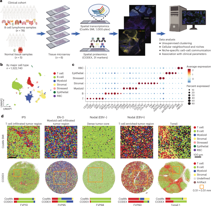
The CosMx SMI data for TMA slides, including gene count matrices, metadata, FOV positions, cellular boundary coordinates and transcript coordinates, were downloaded from the Nanostring AtoMx Spatial Informatics Platform. The gene count matrix was used for transcriptomic analysis with the R software Seurat (v.5.0.1)⁴⁵. Cells with a unique molecular identifier count of less than 20 or a gene count of less than ten were filtered out. Furthermore, cells lacking the expression of defined canonical markers were excluded from subsequent analyses. Finally, a total of 1,322,740 high-quality, characterizable cells were retained for downstream analysis, with a median gene count of 74 per cell and a median unique molecular identifier count of 121 per cell. Data normalization was performed using the SCTransform function in Seurat⁴⁵. Linear dimension reduction based on highly variable genes was performed by principal component analysis (PCA), using the RunPCA function in Seurat⁴⁶. Elbow plots were generated using the ElbowPlot function, and the number of dimensions used for downstream analysis was determined accordingly. Following this step, TMA-specific batch effects were evaluated, and data integration in the PCA space was performed using the R package Harmony (v.0.1.1)⁴⁷. A nearest-neighbor graph was then constructed with the FindNeighbors function in Seurat⁴⁵, and unsupervised cell clustering was conducted using the Louvain algorithm with the FindClusters function. At a resolution of 0.1, a total of 19 cell clusters were identified. Further non-linear dimension reduction was performed using the uniform manifold approximation and projection method⁴⁸, implemented with the RunUMAP function in Seurat⁴⁵.

Cell type and state identification

DEGs among cell clusters were identified using the FindAllMarkers function in Seurat⁴⁵. The top DEGs of each cell cluster were manually reviewed. Additionally, the expression levels of canonical lineage markers, as reported previously^17,49,50,51, were manually checked, and dot plots were generated using the DotPlot function in Seurat⁴⁵. Based on these methods, cell clusters were annotated as T cells and natural killer cells (high expression of CD3D, CD3E, CD2 and so on), B cell and plasma cells (high expression MS4A1, CD79A, MZB1 and so on), myeloid cells (high expression of CD68, APOE, C1QB and so on), stromal cells (high expression of COL1A1, COL1A2 and so on), stressed cells (high expressing of HSP genes), epithelial cells (high expression of KRT genes) and erythrocytes (that is, red blood cells) (high expression of HBB, HBA1/2).

To further validate the accuracy of the identified cell types, the signatures of major cell types from an in-house-constructed B cell lymphoma atlas were used (see Supplementary Table 4 for the detailed signature). This atlas was based on single-nucleus RNA sequencing (snRNA-seq) data from 105 B cell lymphoma samples and contained 970,239 cells, ensuring its comprehensiveness and accuracy as a reference. Signature scores for each major cell type were calculated using the AddModuleScore function and visualized with the FeaturePlot function in Seurat⁴⁵. Furthermore, we integrated the CosMx SMI and single-nucleus RNA sequencing datasets using Harmony⁴⁷ and overlaid the two datasets in the joint embedding space for all cells as well as for each major cell type. Finally, we performed Spearman correlation analysis to evaluate the concordance of major cell types identified from CosMx SMI and CODEX datasets using the same set of samples.

Identification of cellular neighborhoods and spatial niches

We defined a cellular neighborhood as the collection of cells whose centroid lies within 200 pixels (24 µm) of the centroid of the center cell. Such a strategy was applied to the entire CosMx SMI dataset, with each retained high-quality cell being iteratively selected as the center. Based on this definition, most cellular neighborhoods contain ~10–20 cells. A cell-by-cell state composition matrix was then calculated, in which each column represents a center cell and each row represents the count of a cell state within that center cell’s neighborhood. We tested multiple neighborhood radii (from 100 pixels to 2,000 pixels) and obtained the corresponding neighborhood composition matrix. Then, pairwise Spearman correlation analysis was performed to assess the similarity of the neighborhood structures obtained using different neighborhood searching radii.

Subsequently, k-means clustering was performed based on the cell-by-cell state composition matrix, obtained using a neighborhood radius of 200 pixels, to cluster center cells based on the similarity of their neighborhood structures. Multiple resolutions were tested to optimize the clustering results. Then, clusters with similar structures were combined to reduce redundancy. This analysis identified seven cell clusters, each characterized by unique neighborhood compositions, which we defined as spatial CNs. Dimensionality reduction of the dataset was performed on the scaled neighborhood compositions using PCA, and the CN information was projected onto the PCA space for visualization.

Quantification of cellular enrichment

To quantify the enrichment of different cell states across different groups (that is, the neighborhood compositions of different cell states or the cellular compositions of different spatial niches) and determine whether a certain cell state is enriched or depleted, we calculated the ratio of observed to expected cell numbers for each cell state across different groups, as reported previously⁵². First, a contingency table of cell states by groups was calculated. Then, a chi-squared test was performed to calculate the expected distributions of cell states across the different groups and to evaluate the deviation of the actual distribution from the expected distribution. Following this, the R_o/e values for each cell type-group combination were calculated using the following formula:

Here, R_o/e represents the ratio of observed to expected cell numbers for a particular cell state within a given group. For a specific cell state, R_o/e > 1 indicates that cells of this state are observed more frequently than expected by random chance in that group (that is, enriched), whereas R_o/e < 1 indicates that the number of cells of this state is lower than expected (that is, depleted). The results were shown as heatmaps using the R package pheatmap (v.1.0.12).

Niche-specific cell co-localization network

The cell co-localization network in each spatial niche was calculated with the R package CellTrek (v.0.0.94)⁵³. In brief, the function scoloc was used to construct a minimum spanning tree based on the Delaunay triangulation network for cells within each spatial niche. The co-localization graph of different cell states within each spatial niche was then visualized using the function scoloc_vis. In the graph, each node represents a cell state, and the width of the edge connecting two cell states represents their proximity within the specific niche.

Niche-specific cell functional state analysis

The FindAllMarkers function in the R package Seurat⁴⁵ was applied to identify DEGs for different spatial niches as well as DEGs for specific cell types across different spatial niches. Specifically, the cell cycle signature was derived by intersecting the cell cycle metaprograms reported in a recent pan-cancer study⁴⁶ with the CosMx SMI gene panel (see Supplementary Table 6 for the detailed signature). The T cell cytotoxicity and exhaustion signatures were derived by intersecting the DEGs of corresponding cell clusters from a pan-cancer T cell atlas¹⁷ with the CosMx SMI gene panel. The top 20–50 DEGs from the pan-cancer T cell atlas were used for constructing each signature, ensuring that at least ten genes overlapped with the CosMx SMI gene panel (see Supplementary Table 9 for the detailed signature). The signature scores were then calculated using the AddModuleScore function in Seurat⁴⁵.

Neighborhood-based cell–cell communication analysis

For spatially resolved single-cell transcriptomic data, we inferred cell–cell communications within each cell’s neighborhood, leveraging spatial information and restricting cellular communication to adjacent regions. We used the human ligand–receptor databases from CellChat⁵⁴, CellPhoneDB (v.2.0)⁵⁵ and iTALK⁵⁶, which together comprised a total of 4,028 ligand–receptor pairs. The crosstalk between each cell and its neighboring cells was quantified based on ligand–receptor interaction activity, calculated as follows:

where L stands for a ligand, R stands for the corresponding receptor, s denotes a sender cell expressing ligand L, r represents a receiver cell expressing the corresponding receptor R, Exp_L,s stands for the expression value of ligand L in the sender cell s and Exp_R,r stands for the expression value of the corresponding receptor in the receiver cell r. The calculations described above were implemented using the commu.cn.call function in Spyrrow (v.0.1; https://github.com/liuyunho/Spyrrow) in the Python environment (v.3.10.5). The results were visualized using the ggplot2 package (v.3.4.4) in R (detailed in the section ‘CosMx SMI data visualization’).

Calculation of normalized PD-L1–PD-1 interaction count and intensity

The normalized PD-L1–PD-1 interaction count was calculated as the total number of cell pairs of interest (myeloid–T cell pair or tumor–T cell pair) with a positive PD-L1–PD-1 interaction activity, divided by the total number of receiver cells (C5_T plus natural killer cells) in each spatial niche. The normalized PD-L1–PD-1 interaction intensity was calculated as the sum of PD-L1–PD-1 interaction activity between cell pairs of interest (myeloid–T cell pair or tumor–T cell pair) divided by the total number of receiver cells (C5_T plus natural killer cells) in each spatial niche. These two matrices assess the extent to which T cells were influenced by the PD-L1–PD-1 interaction in each spatial niche.

CosMx SMI data visualization

Cell patch plots were generated using the cell boundary coordinates, implemented with the function plot_cell_patch in the software Spyrrow. The single-molecule resolution gene expression plots were generated using both the cell boundary and transcript coordinates by plotting the transcripts on top of the corresponding cell patches. This was implemented with the plot_RNA_on_cell function in Spyrrow, with the transcripts plotted only for the cell states of interest. For the visualization of cell–cell communication results, the R package ggplot2 (v.3.4.4) was applied. For the communication between cell clusters in one or different spatial niches, dot plots were applied to show the proportion of cell pairs involved in the specified ligand–receptor interaction in a certain niche and the average interaction intensity (total interaction intensity normalized by the number of cell pairs).

CODEX assay

CODEX technology (Akoya Biosciences) was used for multiplex immunofluorescence marker detection on FFPE tissue sections.

Antibody conjugation

In addition to the commercially available conjugates from Akoya Biosciences, additional antibody conjugates were made in-house using barcodes and conjugation kits provided by Akoya, following the manufacturer’s protocol. In brief, each antibody in purified, carrier-free form was treated with the reduction solution (conjugation kit component) to open up the thiol groups and subsequently incubated with a unique DNA barcode for 2 h. Successful conjugations were first confirmed with a gel electrophoresis run, showing an upward shift in molecular weight. These conjugates were then tested at different dilutions for staining on a sample tissue expressing the target antigen. The staining was reviewed and approved by pathologists. A comprehensive list of the antibody conjugates used in this study, including the conjugates from Akoya, is provided in Supplementary Table 3.

Tissue staining

Tissue staining and imaging were performed according to the instructions by Akoya Biosciences. In brief, FFPE sections (4 μm thickness) mounted on coverslips were baked at 55–60 °C overnight. Once cooled down to room temperature (20–25 °C), the slides were rinsed in deionized water, followed by rinses in CODEX hydration buffer, and then placed in staining solution to incubate at room temperature for 30 min. Then, 200 μl of antibody conjugate mix consisting of CODEX staining solution, blocking solutions and antibody conjugates at different dilutions (see Supplementary Table 3) was added onto the tissue section and incubated for 3 h at room temperature. After incubation, the coverslips were washed in staining solution twice, post-fixed with 1.6% paraformaldehyde in storage buffer, cold 100% methanol and an Akoya final fixative with abundant washing steps in 1× PBS in between and after each step. The coverslips were then subject to imaging or short-term storage in storage solution at 4 °C for up to 5 days.

Imaging on the CODEX instrument

A 96-well reporter plate containing the corresponding reporters was prepared for imaging. Each well to be used in the plate contained three reporters that correspond to the antibodies used in each cycle, plus a DAPI nuclear stain. Two wells containing only DAPI were used as the first and last cycle for the correction of background, known as blanks. The plate was sealed with a foil plate seal to block it from light. During imaging, one coverslip was mounted on a perfusion stage resting on a Keyence fluorescence microscope (model BZ-X800) equipped with a ×20/0.75 NA objective. The solution exchanges were performed using a microfluidics instrument (Akoya Biosciences) and controlled through a software interface. The order of markers per cycle is listed in Supplementary Table 3. After completion of imaging cycles, the raw image tiles in.tiff format were fed through the CODEX image processor for stitching. Quality control of tissue, signals and staining was performed by an experienced pathologist.

CODEX data analysis

Cellular segmentation

Cellular segmentation was performed using a convolutional neural network-based approach with UNet++ architecture. As inputs, the nuclear marker DAPI and the most common membrane marker Na/K-ATPase were used. A cell instance mask, which includes each cell detected by the aforementioned network, was produced as an output of the cellular segmentation process. Cell instances that lack clearly visible membranes but contain nuclei were segmented with a slight extension around the nuclei. The segmentation quality for all samples was visually inspected by pathologists experienced in MxIF analysis. It was confirmed that the segmentation quality for all cores met the 90% threshold. To ensure accurate analysis, large segments that did not represent real cells and appeared as a result of artificial staining, blur or other artifacts were filtered out based on their size.

Mask generation

Signal masks for macrophages were generated by setting a threshold for CD68, CD11c, CD206 and HLA-DR markers. Vessel masks were generated with UNet++ with an EfficientNet-v2 encoder using SMA, CD31 and nucleus (DAPI/DRAQ5) markers. For cases in which results were unsatisfactory (that is, more than 10% of the signal area was lost or more than 10% of the detected area did not belong to the correct compartment or cell population), masks were corrected manually.

Cell typing

Cell classification was performed based on the expression of each marker and the distribution of markers in the cell’s contour, such as the cells’ mean marker intensity. Cell typing was performed across the entire set of cells in the analysis. A batch-balanced k-nearest neighbor tree⁵⁷ was constructed, and further clustering was performed using the Leiden algorithm⁵⁸ along with the Wilcoxon signed-rank test to assign specific cell types to the clusters. To ensure cell typing accuracy, a ‘gating’ strategy was used to verify that detected clusters of cells with a given phenotype did not contain cells lacking expression of the specified marker or any other inconsistencies with the assigned phenotype. This was achieved by comparing marker expression levels to a ‘threshold’ value, which was determined either through manual review of the image data or by inferring the value from the distribution of the given cluster.

A two-step strategy was then applied for cell typing. In the first step, major cell types were identified, including B cells (cells expressing CD45 along with one of the markers CD19, CD20 or CD79a), T cells (CD45⁺CD3⁺CD4⁺, CD45⁺CD3⁺CD8⁺ and CD45⁺CD3⁺FOXP3⁺ cells), macrophages (CD68⁺ cells), endothelial cells (CD31⁺) and stromal cells (FN1⁺ or SMA⁺). These major cell types were cross-validated by two experienced pathologists to ensure alignment with the observed fluorescent signals. In the second step, cell subtypes were identified: B cells were subdivided based on co-expression of CD10, CD21, CD23 or Bcl2; T cells were classified based on co-expression of PD-1, ICOS (for CD8⁺ and CD4⁺ cells) or Granzyme B (for CD8⁺ cells); and macrophages were subdivided based on co-expression of CD206. After identifying the detailed cell subtypes, all cell classifications were re-evaluated by pathologists to confirm accuracy.

Statistics and reproducibility

Comparisons of cellular and CN compositions between EBV-positive and EBV-negative nodal lesions were performed using the Wilcoxon rank sum test. Comparisons of cellular and CN compositions among different tumor anatomical sites were done with the Kruskal–Wallis test, with intergroup comparisons performed using Dunn’s test for multiple comparisons, applying the Holm method to adjust P values. For comparisons of signature score expressions between EBV-positive and EBV-negative nodal lesions, the Student’s t-test was conducted. Pairwise t-tests were used for comparisons of signature score expressions among different tumor sites, with the Benjamini–Hochberg method used to control the false discovery rate. For comparisons of individual gene expression levels among different clinical groups, the P values were obtained using the FindAllMarkers function in Seurat⁴⁶, using the default Wilcoxon rank sum test. For all comparisons described above, two-sided P values were reported, and P < 0.05 was considered statistically significant. Unless otherwise specified, all bioinformatic and statistical analyses in this study were implemented in the R statistical environment (v4.2.0; https://www.r-project.org).

Sample size of the study was determined based on the sample availability. No statistical methods were used to determine sample size. All statistical comparisons were made using data from all applicable cases, with sample sizes described in the Results section and assignment of patients for each comparison group outlined in Supplementary Table 1. No data were excluded from the analyses, and the experiments were not randomized. Investigators were blinded to sample characteristics during data acquisition and processing. Individual cases were selected for display in figures based on their alignment with the overall trend from the full series.

Whole-exome sequencing and bulk RNA sequencing

A full description of the methods for whole-exome sequencing and RNA sequencing can be found in the Supplementary Information.

Reporting summary

Further information on research design is available in the Nature Portfolio Reporting Summary linked to this article.