Single-cell and isoform-specific translational profiling of the mouse brain

Molecular cloning and AAV production

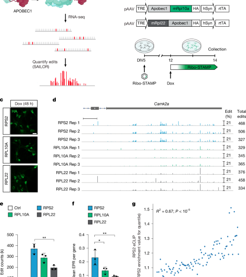
The original Ribo-STAMP construct consisted of a Tet-On hRPS2–APOBEC lentiviral expression vector, with a human phosphoglycerate kinase (PGK) promoter driving the expression of rtTA and pac, designed for generation of stable human cell lines¹⁸ (Fig. 1b). ORFs of Ribo-STAMP variants were first cloned into a plasmid derived from the pLIX_403 vector (a gift from D. Root; Addgene plasmid no. 41395) containing a P2A-mRuby fluorescent protein sequence in-frame with the fusion protein. The RPS2–APOBEC fusion sequence was taken from the pLIX403_Capture1_RPS2_APOBEC_HA_P2A_mRuby construct, as used previously¹⁸. Following the EGFP-tagging methodology of the TRAP system⁶¹, the ORF isoform 1 of the mouse Rpl10a was fused to the C terminus of APOBEC1. A similar strategy was adopted for the Rpl22–APOBEC fusion sequence whereby the mouse Rpl22 ORF was fused to the N terminus of APOBEC to mimic the haemagglutinin-tagging strategy of RiboTag⁶². Both fusion sequences were generated as synthetic gBlocks (Integrated DNA Technologies) and cloned into the pLIX403_Capture1_APOBEC_HA_P2A_mRuby parental backbone using Gibson assembly. The Tet-On Ribo-STAMP constructs used in Figs. 1 and 2 were cloned into a mammalian gene expression AAV vector (VectorBuilder) containing a truncated woodchuck hepatitis virus post-transcriptional regulatory element (WPRE) and bovine growth hormone polyadenylation signal (BGH polyA), using Gibson assembly. The tetracycline-responsive promoter element, followed by Ribo-STAMP variant ORFs, was polymerase chain reaction (PCR)-amplified from the previously described plasmids. The hSyn promoter was PCR-amplified from pAAV.Syn.GCaMP6s.WPRE.SV40 (a gift from D. Kim; Addgene plasmid no. 100843), and the rtTA was PCR-amplified from the pLIX_403 vector. Ribo-STAMP constructs used in Figs. 1 and 2 were cloned into a mammalian gene expression AAV vector (VectorBuilder). Constitutive RPS2-STAMP used for in vivo experiments was assembled by VectorBuilder. The construct was cloned into a mammalian gene expression AAV vector (VectorBuilder) containing an EF1A promoter, the RPS2_APOBEC ORF containing an haemagglutinin tag as above and fused with TdTomato through a P2A peptide, followed by a truncated WPRE and BGH polyA. AAVs were prepared following Challis et al.⁶³ using the PHP.eB capsid for packaging.

Animals

C57BL/6J mice were group-housed on a 12-h light–dark cycle and fed a standard rodent chow diet. All experimental protocols were approved by the Institutional Animal Care and Use Committee at Scripps Research Institute and were in accordance with the guidelines from the National Institutes of Health (NIH).

Primary neuron culture, treatments, infections and viability test

Cortices were dissected from E18 C57BL/6J embryos in Leibovitz’s L-15 Medium (Life Technologies) and incubated in TrypLE Express (Life Technologies) at 37 °C for 4 min. Neurons were mechanically dissociated and plated on poly-d-lysine-hydrobromide-coated six-well plates (600,000 cells per well) or on 12-mm coverslips in 24-well plates (100,000 cells per well). Neurons were maintained in a humidified environment at 37 °C and 5% CO₂ in neurobasal medium (Life Technologies) supplemented with B27 Plus Supplement (Life Technologies) and GlutaMAX (Life Technologies). At day in vitro (DIV) 3, floxuridine was added to the medium to limit the growth of dividing cells. DIV 6 neurons were infected with 1 × 10¹³ (24-well plates) or 4 × 10¹³ (six-well plates) viral genomes ml⁻¹ of inducible Ribo-STAMP AAV virions. Ribo-STAMP expression was induced with 1 µg ml⁻¹ Dox for 48 h before collection at DIV 14. BDNF (100 ng ml⁻¹) was applied 15 min and 60 min before collection^64,65. Anisomycin (40 µM) was applied 30 min before collection. For Puro-PLA experiments, neurons were treated with puromycin (10 μm) for 15 min before collection. Cell viability assay was performed using the Cell Counting Kit Assay-8 (MilliporeSigma).

Proximity ligation assay

Proximity ligation assay (PLA)⁶⁵ was performed using the Duolink kit (Sigma). After puromycin treatment, neurons were washed in PBS, fixed for 10 min in 4% paraformaldehyde (PFA) and washed again in PBS. Fixed neurons were permeabilized with 0.1% Triton X-100 in PBS-CM (PBS (pH 7.4), 1 mM MgCl₂ and 0.1 mM CaCl₂) for 10 min. All reactions were incubated in a preheated humidity chamber. After a brief wash with PBS-CM, each sample was blocked with Duolink Blocking Solution for 1 h at 37 °C and then incubated with anti-puromycin and protein-of-interest primary antibodies diluted in Duolink Antibody Diluent overnight at 4 °C. After two washes in wash buffer A, PLA rabbit plus and mouse minus probes were applied at a 1:5 dilution in Duolink Antibody Diluent for 1 h at 37 °C. After washes, ligation and amplification reactions were performed using Duolink Fluorescent Detection Reagent in FarRed. The cells were incubated in the ligation reaction for 30 min at 37 °C, washed with wash buffer A and incubated in the amplification reaction for 100 min at 37 °C. Following the final washes with 1× and 0.01× wash buffer B, cells were postfixed for 10 min with 4% PFA, washed in PBS and prepared for immunocytochemistry.

Immunocytochemistry

PFA-fixed cells were permeabilized with 0.1% Trixon-X 100 in PBS for 10 min at room temperature, washed in PBS and blocked with 10% normal goat serum (NGS) in PBS for 1 h at room temperature. Cells were incubated with primary antibodies at desired concentrations in 1% NGS in PBS overnight at 4 °C. After three washes with PBS, cells were incubated with secondary antibodies at 1:500 dilution in 1% NGS in PBS for 2 h at room temperature. After three washes with PBS, coverslips were mounted onto microscope slides (Thermo Fisher Scientific) with ProLong Diamond Antifade Mountant (Life Technologies) and imaged.

Immunocytochemistry image acquisition and analysis

Representative images in Fig. 1 and Extended Data Fig. 1 were acquired with a Nikon A1 confocal microscope at a 1,024 × 1,024 resolution using a Plan Apo VC 20× DIC N2 objective through the thickness of the neurons (five stacks; 3.2 µM step size). To assess AAV infection, stitched images of four fields were acquired with a Plan Apo 10× DIC L objective, and the percentage of Ribo-STAMP over NeuN-positive neurons was assessed with CellProfiler.

Puro-PLA

Z-stack images were acquired with a Nikon A1 confocal microscope using a PlanApo ×60 oil, numerical aperture 1.4 objective at a 2,048 × 2,048 resolution throughout the thickness of the neurons (nine stacks; 1.2 µM step size). Five fields within each coverslip were captured, and imaging settings were maintained constant within experiments. Quantification was on the basis of a previous study⁶⁵, with minor modifications. Maximum intensity projections were generated, and manual thresholds were applied to the PLA and MAP2 images using the same values across all samples. In the MAP2-thresholded image, a circular region of interest with a radius of 75 µm, centred on the neuron soma, was selected for quantification, and a mask of the cell body was generated. The mask was dilated by a radius of 2.5 px to include the signal in spines and presynaptic terminals. For each neuron, the area of the dilated MAP2 mask and the area covered by PLA-positive pixels within the mask were quantified. Quantifications are shown as percentage of PLA area over the dilated MAP2 mask area. Statistical tests were performed using GraphPad Prism v.10.2.

FUNCAT and immunolabelling

The non-canonical amino acid AHA was dissolved in ultra-pure water, and the pH was adjusted to 7.4. PTZ was dissolved in Dulbecco’s phosphate-buffered saline at 5 mg ml⁻¹, and the solution was freshly prepared before injections. P25 C57BL/6 male mice were co-injected intraperitoneally with 100 µg gbw⁻¹ AHA (added with 10× PBS) and 8.5 µl gbw⁻¹ PTZ or 1× PBS. PTZ-treated animals exhibited severe seizures. After 18 h, the mice were anaesthetized with isoflurane and intracardially perfused with PBS, followed by 4% PFA. Brains were postfixed overnight in 4% PFA, washed twice in PBS and cut into 50-μm-thick slices using a vibratome (Leica VT1000S). Click labelling was performed on the basis of the published CATCH protocol, with minor modifications⁶⁶. Slices were incubated in 1 mM CuSO₄ in ultra-pure water overnight at room temperature with gentle agitation. The slices were transferred in 150 µM CuSO₄, 300 µM BTTP, 10% dimethyl sulfoxide and 5 μm of AF647 Picolyl Azide in PBS. To kickstart the click reaction, NaAsb was added to a final concentration of 2.5 mM, and the reaction was incubated for 1 h at room temperature with gentle agitation. The reaction was quenched with 4 mM EDTA in PBS (pH 8) and then washed three times in 0.2% Triton X-100 in PBS for 10 min at room temperature. Brain slices were further prepared for IHC.

Immunohistochemistry

Brain slices (50 μm thick) were blocked in 10% NGS and 0.25% Triton X-100 in PBS for 1 h at room temperature. Slices were incubated in primary antibodies at the desired concentrations in 1% NGS and 0.25% Triton X-100 in PBS overnight at 4 °C on an orbital shaker. After three washes in 0.1% Tween in PBS, the slices were incubated in secondary antibodies at a 1:500 dilution in 1% NGS and 0.25% Triton X-100 in PBS for 2 h at room temperature on an orbital shaker. After three washes in 0.1% Tween in PBS, the slices were mounted on slides with ProLong Diamond Antifade Mountant.

IHC acquisition and analysis

Dorsal hippocampus images were acquired in the CA1b and CA3a subfields with a Nikon A1 confocal microscope using a PlanApo ×60 oil, numerical aperture 1.4 objective at a 2,048 × 2,048 resolution. Imaging settings were maintained constant within experiments. For each CA1 and CA3 image, the plane with the brightest signal was selected for quantification. Regions of interest of cell bodies were manually drawn using the NeuN signal as a mask. The mean fluorescence intensity of the analysed proteins within the NeuN mask was measured using Fiji. Interneurons identified through GAD67 staining were excluded from the analysis. Statistical tests were performed using GraphPad Prism v.10.2.

Ribosome structure analysis

The mouse ribosome structure and the relative location of RPS2, RPL22, RPL10a, transfer RNA (tRNA) and mRNA were accessed from Protein Data Bank (PDB) 7CPU⁶⁷, 6Y0G⁶⁸ and 7LS2 (ref. ⁶⁹). Most of the ribosome structure representation, including ribosomal RNA, tRNA, RPS2, RPL22 and most of the other ribosomal proteins, was generated from PDB 7CPU. Owing to the lack of RPL10a and mRNA on PDB 7CPU, PDB 6Y0G and 7LS2 were superimposed to PDB 7CPU to model the structure and the relative locations of mRNA and RPL10a, respectively. All structure superimposition and figure generation were performed using PyMol (https://www.pymol.org/).

eCLIP sequencing

eCLIP sequencing was performed following established protocols⁷⁰. Anti-RPS2 antibody (Bethyl A303-794A) was used. Total RNA was taken from samples before starting immunoprecipitation. ribosomal RNA depletion was performed after library preparation (Jumpcode Genomics). Single-end sequencing was performed with 20 million reads per sample on an Illumina NovaSeq at the University of California San Diego (UCSD) Institute for Genomic Medicine. FASTQ files were trimmed for indices using cutadapt 1.18. Trimmed FASTQ files were subsequently aligned to the mm10 genome using the STAR alignment software v.2.5.2b, with the flags –outSAMAttributes All, –outFilterMultimapNmax 10, –outFilterMultimapScoreRange 1, –outFilterScoreMin 10, –alignEndsType EndToEnd. For each gene, eCLIP immunoprecipitation read counts were divided by total read counts to derive an eCLIP-based translational efficiency value. Genes were split into 100 EPR quantiles, and for each quantile’s set of genes, a mean EPR and mean eCLIP-derived translational efficiency value were plotted against each other, followed by Pearson correlation coefficient and P-value calculations.

Ribo-STAMP bulk RNA sequencing library preparation and analysis

RNA isolation was performed from n = 3 biological replicates using Direct-zol RNA microprep kit (ZYMO; R2062). RNA quality was measured through RNA ScreenTape Analysis (Agilent) before proceeding to library preparation. Illumina TruSeq Stranded mRNA kit (Illumina; 20020595) was used for library preparations. Sequencing was performed at the Institute for Genomic Medicine at UCSD on an Illumina NovaSeq. Thirty million single-end reads were sequenced per sample. FASTQ files were trimmed for indices using cutadapt 1.18. Trimmed FASTQ files were subsequently aligned to the mm10 genome using the STAR alignment software v.2.5.2b, with the flags –outSAMAttributes All, –outFilterMultimapNmax 10, –outFilterMultimapScoreRange 1, –outFilterScoreMin 10, –alignEndsType EndToEnd. BAM files were processed using the SAILOR⁷¹ pipeline to derive the number of edits per gene. Using a custom in-house pipeline, BAM files were processed using feature counts v.1.5.3 to assess the number of reads aligned to each gene. Both edits per kilobase per million mapped reads (EPKM) and EPR values were calculated for each gene for each sample, using edit counts and read counts derived previously.

Differential transcription versus translation analysis after BDNF

DESeq2 v.1.39.3 was used to calculate RNA log₂FC and P values for the comparisons between the BDNF 15′ and no-treatment and BDNF 60′ and no-treatment conditions. A two-sided t-test was used to compare the three replicates of BDNF 15′ and BDNF 60′ EPR values for each gene with the three replicate values of the no-treatment condition. The log₂FC values were calculated as the log₂ of the mean of the BDNF 60′ or 15′ EPR values, respectively, minus the log₂ of the mean of the no-treatment EPR values. P values were adjusted for multiple hypothesis testing using the Benjamini–Hochberg correction. Dox-induced genes shown in Extended Data Fig. 1c were removed from the analyses. IEGs known to be BDNF-induced and activity-induced were taken from previous studies^72,73. Previously validated BDNF-induced transcripts were taken from published literature^{64,74,75,76,77}.

Gene Ontology analyses

Gene Ontology analyses were performed using clusterProfiler v.4.10.1 (ref. ⁷⁸) in R studio, with the exception of that shown in Fig. 2. For comparisons among gene lists, the compareCluster function was used with fun = enrichGO and pAdjustMethod = BH (Benjamin–Hochberg) and with pvalueCutoff = 0.01 and qvalueCutoff = 0.05. Redundant Gene Ontology terms were removed using the ‘simplify’ function with standard settings and cutoff = 0.7. For CA3 EPR up genes in Fig. 6g, the enrichGO function was used with the same settings as above. All genes detected by scRNA-seq in the cell types subjected to a specific analysis were used as background. Biological Process ontologies were visualized unless otherwise indicated. Identification of enriched synaptic terms from ‘EPR up’ and ‘EPR not up’ genes in Fig. 2g was executed using SynGo⁷⁹, using the ‘brain expressed’ background Gene Set Enrichment Analysis setting of ‘min. gene count per term’ set to five and considering the function (biological processes) readout. The lists of ‘EPR up’ and ‘EPR not up’ unique presynaptic and postsynaptic genes used in Fig. 2i–k were manually extracted on the basis of the presynaptic or postsynaptic ontology terms associated with the genes by SynGO. All synaptic genes in Fig. 2k correspond to all the genes retained by SynGo for analysis in the respective conditions. Dox-induced genes shown in Extended Data Fig. 1c were removed from the analyses.

Stereotactic surgery and single-cell dissociation

Single-cell suspensions from hippocampi were obtained following Hochgerner et al.⁸⁰. Three male P22 C57BL/6J mice were stereotactically injected in the dorsal hippocampus with 800-nl EF1a-Ribo-STAMP virus (2.77 × 10¹³ viral genomes ml⁻¹) bilaterally using the following coordinates (from bregma): anterior–posterior, −2 mm; medial–lateral, ±1.7 mm; and dorsal–ventral, −1.6 mm. All mice were processed separately to maintain independent replicates. P25 mice were anaesthetized 72 h later and intracardially perfused with cold carboxygenated artificial cerebrospinal fluid. Brains were sliced in 300-μm-thick coronal sections. Dorsal and dorso-ventral hippocampi were manually microdissected, incubated in Papain/DNaseI (Worthington dissociation kit) and mechanically dissociated. The resulting single-cell solutions were filtered, centrifuged through a 5% OptiPrep gradient and diluted to a final concentration of 1,200 cells µl⁻¹ for scRNA-seq processing.

Single-cell library preparation and analysis

Single-cell libraries were constructed using the 10x Genomics Chromium Next GEM Single Cell 3′ Reagent Kits v.3.4. The target cell recovery was 10,000 cells per replicate. Single-cell libraries were sequenced at the Genomics Core at The Scripps Research Institute on an Illumina NextSeq200 with a target of 100,000 reads per cell. The 10x FASTQ files were aligned with Cell Ranger v.3.0.0 using a reference transcriptome modified to include mm10 genome and the tdTomato sequence from the Ribo-STAMP construct. Scrublet was used to remove doublets in the data⁸¹. Scanpy was used for single-cell analysis and plotting (https://scanpy.readthedocs.io/en/stable/). Quality control was performed separately on each replicate, as recommended in the Scanpy documentation. All replicates were filtered to remove genes in which fewer than five cells had expression values greater than 0, cells with less than 2,000 genes expressed, cells with more than 10,000 genes expressed and cells with more than five mitochondrial counts. The following filters were used to filter cells on the basis of Gm42418 counts: rep1, Gm42418 less than 7.5; rep2, Gm42418 less than 10; and rep3, Gm42418 less than 15. Counts per million (CPM) and log normalization were used for RNA counts. Batch balanced k-nearest neighbours batch correction was performed on samples using Scanpy⁸². Cell assignments were done using RNA counts using known marker genes^14,83,84.

Single-cell and isoform-level edit calling

Overview

MARINE is a versatile, robust, memory-efficient and ultra-fast Python package we developed to identify RNA edits at single-cell and isoform-level resolution in our dataset (Supplementary Fig. 2a). The modular framework of MARINE includes components for read processing, edit identification and coverage calculation that can be leveraged for both bulk and single-cell processing, with extra features tailored to single-cell data. MARINE is implemented in Python, leveraging pysam for alignment manipulation, pandas and polars for data handling and multiprocessing for parallelization.

Inputs

Any aligned.bam file, whether derived from single-cell or bulk sequencing libraries and using either single-end or paired-end and either short or long reads, can in principle be analysed using MARINE. For single-cell data, a list of valid cell barcodes can be provided as a whitelist, ensuring that only reads associated with recognized cells are included in the analysis. We analysed only the cells not removed during the quality-control filtering step.

Edit calling and filtering

To optimize parallelization in the edit identification step, the input.bam file is divided into smaller regions defined by genomic contigs and intervals, with each region processed independently. MARINE simultaneously tabulates all edit types at all non-reference positions in each cell (or cell–isoform combination) by combining aligned read sequence information with information derived from the mismatch descriptor (MD) and Compact Idiosyncratic Gapped Alignment Report (CIGAR) read tags. Reads are excluded if they fail quality control checks, are unmapped, are unique molecular identifier duplicates (do not contain the xf:25:i tag), represent secondary or supplementary alignments or do not meet user-specified thresholds for mapping quality. Bases are excluded if they fail user-defined filters for base quality or proximity to read ends, in which base quality is known to drop off.

Coverage calculation

MARINE efficiently calculates per-cell coverage information at these positions through reconfiguration of aligned read metadata. Reads are regrouped by chromosome and barcode, and the contig name is modified to include both the genomic region and the cell barcode (for example, chr1_). This modification enables downstream tools such as Samtools82 to treat each cell–barcode pair as a unique entity. Coverage at edited sites is then calculated independently for each cell–barcode pair, quantifying reads supporting reference and alternate bases at every genomic position in cells with the edit.

Benchmarking for accuracy, speed and memory usage

Although earlier tools addressed edits at single-cell resolution⁸⁵, MARINE can rapidly identify barcode-specific edits de novo. Given n edited reads, MARINE operates with a time complexity of O(n) (Supplementary Fig. 2b), whereas memory usage can be capped at a constant O(c) (Supplementary Fig. 2c). Although MARINE can run efficiently on a single CPU, its performance is significantly enhanced when executed across several cores; for systems with limited RAM, MARINE can be throttled to process fewer chromosomes simultaneously, reducing memory requirements at the cost of increased runtime (Supplementary Fig. 2d). Although primarily designed for single-cell data, MARINE boasts a best-in-class balance of speed and memory efficiency when applied to bulk datasets, with memory and time complexity also of O(n) and O(c), respectively. Despite minor differences resulting from algorithm-specific filters, MARINE reliably detects all RNA editing sites identified by both REDItools2 and JACUSA2, two widely used multiprocessing-enabled tools for RNA editing detection (Supplementary Fig. 2e). MARINE achieves runtimes comparable to JACUSA2 while maintaining memory usage similar to REDItools2.0 (Supplementary Fig. 2f,g). At its highest efficiency, with increased core usage, MARINE surpasses both tools in speed and memory efficiency (Supplementary Fig. 2f,g).

Outputs

Depending on parameters, both coverage and edit data can be aggregated into a sparse matrix format, with cell barcodes as rows and genomic positions as columns, enabling integration with single-cell transcriptomic analysis frameworks, such as Scanpy. Outputs include site-level summaries and, optionally, .bedgraph files for visualization in tools, such as IGV, or BED files formatted for downstream tools, such as FLARE.

Short-read EPR pipeline for single cells

Edit sites (sites with more than one edit type) and edits overlapping SNPs found in the dbSNP mm10 database were filtered out, as were edit sites with less than three total edits across all cells, to yield edit counts per cell. Edits and Cell Ranger raw counts were used to compute EPR values for each gene within each cell. Edit sites that mapped to antisense reads were determined by strand-specific intersection with an annotation gtf file and subsequently filtered out. In addition, edits at which more than 5% of reads were edited were filtered out. After these filters, 65%, 62% and 63% of edit sites remaining were C>U for the three replicates, respectively.

The EPR levels for each replicate were normalized to Stamp expression using linear regression. Briefly, for each cell, the mean EPR value was calculated as the sum of EPR values across all edited (with more than zero edits and three or more reads) genes, divided by the number of edited genes. For cells with non-zero Stamp expression, we performed ordinary least squares linear regression, using the log-transformed Stamp CPM counts as the independent variable and the log-transformed mean EPR as the dependent variable:

The regression residuals were extracted and exponentiated to reverse the log transformation and then rescaled and shifted to preserve the original dynamic range and avoid negative values. Rescaling was done by aligning the minimum and maximum of the residual distribution to those of the uncorrected mean EPR. Translation ensured that the minimum corrected EPR matched the original minimum EPR. These regression residuals represent the Stamp-corrected EPR values.

A cell-specific normalization factor was then calculated as the ratio of corrected to original mean EPR. The edit counts of each cell were multiplied by its corresponding factor to produce an adjusted editing matrix. The read count matrix was masked using a minimum read-depth threshold of 5, preserving edit counts only for gene–cell pairs with five or more reads and setting others to zero. Final EPR matrices were recalculated as the ratio of normalized edit counts to unadjusted read counts. Only cells containing at least five edited genes were retained for downstream analysis.

Clustering cells by EPR

To validate that edits were deposited in a cell-type-specific manner, we clustered cells by EPR and evaluated whether these new clusters matched the RNA-based cell assignments. Clustering single cells by EPR was very noisy and not definitive. We reasoned that the sparsity of edits precluded to identify cell types. Thus, to overcome this limitation, we created pseudocells that represented 5, 10 or 15 cells from the same cell-type assignment (on the basis of RNA) randomly grouped. We summed the normalized edit counts and raw read counts. We then calculated EPR as edits/reads for each pseudocell. We repeated this five times to account for variation in the shuffling to create five randomly shuffled EPR datasets. Log normalization, data scaling, principal component analysis, neighbour calculations, UMAP and Leiden clustering were performed. We plotted this in UMAP space for both EPR Leiden clusters and the original cell-type assignments. For cell types with the largest numbers of cells, clustering by EPR replicated the original RNA cell assignments, and the more cells included (15 cells), the clearest clusters separated. Representative UMAPs from one shuffle replicate are shown in Extended Data Fig. 5. All five shuffle replicates yielded similar results.

Differential EPR analysis across all cell types

Differential expression analysis was done for EPR using Scanpy’s rank gene groups with groups=‘all’, reference=‘rest’ and method=‘wilcoxon’ to find EPR marker genes (Fig. 3e). For each annotated cell type, genes with a positive log-fold change and P < 1 were considered. To ensure specificity, we excluded genes that were also significantly expressed (P < 0.05) in any other cell type. The remaining genes were sorted by their ranking score, and the top 3 genes per cell type were selected for dot-plot visualization. For Gene Ontology enrichment analysis, the top 100 genes by ranking score were used per cell type.

EPR relationship to RNA

Cell-type analysis

Pseudobulk EPR and RNA counts were calculated before correlations and clustering. To compute pseudobulk EPR and RNA counts, we processed single-cell data grouped by cell type and sample. A minimum raw read threshold of 5 was applied to filter low-coverage gene–cell observations. For each unique combination of cell type and sample, total EPR was calculated across cells as the sum of edits divided by the sum of raw reads per gene. The mean of total EPR was then calculated across samples per cell type for downstream analysis. All cell types were merged into one dataframe. Next, we applied a multistep filtering procedure to remove genes with low reads or edits. For each gene, we required that at least one cell type exhibited sufficient coverage across all samples. Specifically, we retained genes when (1) total reads were five or more in all samples of at least one cell type; (2) total edits were five or more in all samples of at least one cell type; and (3) at least one cell per sample passed the read threshold in at least one cell type. These conditions were applied to a multi-indexed dataframe containing pseudobulk metrics per gene, cell type and sample. The final filtered matrix included only genes passing all three criteria. For each unique combination of cell type and sample, total counts were calculated across cells as sum of normalized counts per gene, and mean counts were calculated across cells as mean of normalized counts. Normalized counts refer to CPM and log normalization. The mean of total counts (total normalized counts) and mean of mean counts (mean normalized counts) were then calculated across samples per cell type for downstream analysis. Spearman correlation was performed between pseudobulk EPR and pseudobulk total normalized RNA counts and visualized using a seaborn.heatmap() (Fig. 3f). To visualize EPR of all genes across cell types (Extended Data Fig. 5c,d), we used seaborn.clustermap() with settings standard_scale=‘row’ and metric=‘braycurtis’ for pseudobulk EPR. To visualize RNA counts in the same order as EPR, we used pseudobulk RNA mean normalized counts with settings standard_scale=‘row’ and clustering turned off.

Oligodendrocyte analysis

Pseudobulk EPR and RNA normalized total counts for oligodendrocytes were computed as described above. Genes were retained only if they met the following criteria across all samples: (1) total reads of five or more; (2) total edits of five or more; and (3) at least five cells passing the minimum read threshold. To identify and visualize clusters of similarly expressed genes, we applied agglomerative hierarchical clustering to a merged dataset of pseudobulk EPR and RNA normalized total counts. Pairwise distances between rows were computed using the Bray–Curtis dissimilarity metric. Clustering was performed using the AgglomerativeClustering algorithm⁸⁶, with average linkage and a precomputed distance matrix. A manual number of clusters (n_clusters = 8) was specified to reflect visual patterns. Clusters were visualized using seaborn.clustermap(). A scale factor of 1,000,000 was multiplied to EPR values to ensure similar scaling next to RNA counts for visualization.

Translational cell state analysis

Identifying translational cell states

CA1.2 and CA1.4 were annotated as high translation and CA1.1 and CA1.3 as low translation manually by using RNA cell assignments. To categorize CA3 cells into high and low translation groups on the basis of editing rate, we used Gaussian mixture modelling. Specifically, we applied Gaussian mixture modelling with two components to the per-cell total editing rate, calculated as the ratio of total edits to total reads. The model was fit using the GaussianMixture implementation from scikit-learn (n_components = 2; random_state = 42). Cells were then assigned to one of two clusters on the basis of the maximum posterior probability. The cluster with the higher mean was designated as the high group and the other as the low group. For CA3 filtering, cells were retained between 0.65 and 0.80 quantiles on the basis of Ribo-STAMP RNA counts.

Differential gene expression analysis using scanpy.tl.rank_genes_groups was performed with EPR between high and low groups for CA1 and CA3 to identify genes undergoing translation in the high groups. The statistical method used was ‘Wilcoxon’. For bursty gene analysis, CA1 subfield marker genes^4,87 and bursty marker genes⁸⁸ were used.

Differential EPR versus RNA analysis between CA3 and CA1

To identify genes with differential translation between CA3 and CA1 neurons, we analysed EPR across several biological replicates. For each replicate, genes were retained for analysis if they had editing events (EPR > 0) in at least two cells. Cells were retained for each gene if they had a minimum of five raw reads.

For each gene in each replicate, we computed the sum of edits and raw reads across CA3 and CA1 cells, respectively. EPR was then calculated as the total number of edits divided by the total number of raw reads per cell type. For downstream analysis, we included only genes with non-zero EPR values in all three replicates.

Mean EPR was computed across replicates and used for log₂FC of translation for CA3 compared with CA1 neurons (log₂[CA3_EPR/CA1_EPR]). To assess statistical significance, we performed vectorized bootstrap resampling (n = 10,000 iterations). In each iteration, the EPR values across replicates were resampled with replacement and randomly reassigned to CA3 or CA1 group. The test statistic was the mean EPR difference across conditions. Empirical P values were calculated on the basis of the fraction of bootstrap samples with a mean difference greater than or equal to the observed statistic.

For differential count expression analysis between CA3 and CA1, we used scanpy.tl.rank_genes_groups.

For mean EPR of CA3 EPR upregulated ribosomal proteins of the small (RPS) or large (RPL) subunits and translation factors in CA1 and CA3 neurons shown in Fig. 6h, the mean EPR across replicates was used.

CA3/CA1 Ribo-STAMP correlations to existing datasets

The ratio of CA3 EPR to CA1 EPR for each gene was calculated in terms of log₂FC. Existing datasets were standardized for comparison as follows: (1) For RiboTag¹⁶, no further processing was necessary. The precalculated CA3/CA1 log₂FC value was used from this dataset to make our comparisons with EPR. (2) For RIBOmap/STARmap²⁷, RTE was calculated as the ratio of RIBOmap and STARmap signals from sequential brain slices across all genes. RTE for each gene was calculated for CA3 and CA1, and then a log₂FC quantity was calculated for the ratio of CA3 RTE to CA1 RTE. (3) For human hippocampus mass spectrometry dataset⁸⁹, the precalculated log₂FC of CA1/CA3 grouped abundances was inverted (*−1) to obtain a comparable CA3/CA1 log₂FC value for each gene. Correlation plots were made in which the x axis represents a cell count filter, such that at each location along the axis, only genes expressed in at least that number of cells in both CA1 and CA3 were used to calculate the Spearman correlation coefficient. Additionally, genes were retained for the analysis if EPR changes between CA3 and CA1 yielded P < 0.05. The permutation test involved calculating correlations using 100 random shuffles of EPR values within each cell count threshold-derived gene subset.

Single-cell long-read library preparation and analysis

MAS-seq library preparation

Single-cell MAS-seq libraries of single-cell hippocampal RPS2-STAMP complementary DNA (cDNA) generated from the 10x Genomics 3′ kit (10x Genomics; v.3.1; PN-100026) were prepared for long-read single-cell sequencing using the MAS-seq for 10x Single Cell 3′ Kit (Pacific Biosciences; 102-659-600; protocol v.1.03) with the following modifications. To increase library yield while mitigating amplification artefacts, we increased the MAS–PCR volume to 50 µl and the input purified cDNA to 80 ng and decreased the PCR cycle number to seven cycles. Following MAS–PCR, the SMRTbell cleanup bead ratio (Pacific Biosciences; 102-158-300) was altered from 1.5× bead addition volume to reaction volume to 1.35×. Finally, post-array ligation, post-DNA damage repair and final cleanup were purified with a 1.55× SMRTbead cleanup. Following MAS library construction, libraries were quantified with a Qubit dsDNA High Sensitivity Assay Kit (Thermo Fisher Scientific; Q32854) and a Femto Pulse (Agilent; FP-1002-0275). Libraries were sequenced on one 25M SMRT cell (102-202-200) on the Revio platform of Pacific Bioscience.

MAS-seq data processing

The raw HiFi reads generated had average read lengths around 14 kb across 16-mer MAS arrays for all replicates. HiFi reads are circular consensus reads with 90% of bases having Q30 or higher and a median read accuracy of Q30 or higher. These HiFi reads were processed to extract de-concatenated or segmented reads (S-reads) representing the original cDNA sequences, using the SKERA tool of PacBio (https://skera.how/).

Reads were processed in accordance with the PacBio single-cell workflow (https://isoseq.how/umi/high-level-workflow.html) to obtain reads with corrected cell barcode (CB) tags. Deduplication was completed using isoseq groupdedup (v.4.2.0) with default parameters. Reads were filtered to include only those with barcodes assigned to a cell type in the short-read data using samtools view (v.1.18) with parameters -h -D CB. Note that the long-read sequencing barcodes are the reverse complement of the short-read sequencing barcodes. Pbmm2 align (v.1.16.1) was then used to align the reads using the Cell Ranger mm10 reference annotation with the parameter –sort. Samtools (v.1.18) calmd was used to add mismatch descriptor tag. The mismatch descriptor tag is a tag contained within the aligned BAM file that contains information regarding mismatched and deleted reference bases. We use this tag to call edits. Samtools view (v.1.18) was used to filter reads to include only primary alignment reads using the parameter -F 2316.

Reads were assigned to annotated isoforms and their expression quantified using IsoQuant⁸⁵ (v.3.3.0) with parameters –data-type pacbio, –transcript_quantification unique_only and –gene_quantification unique_only. The read assignment output from IsoQuant, together with a custom script, was used to add isoform tags ‘IB’ and ‘IS’ for each read, indicating the isoform to which it was assigned. For this proof-of-concept study, we elected to focus only on annotated isoforms to ensure reliable results.

Long-read edit calling and analysis

MARINE was used to find C>T edit loci for each read. Subsequently, C>T edits were aggregated by isoform to assess isoform-specific edits. Edited sites were removed if they were found among annotated mm10 SNPs obtained from dbSNP. Cell types were assigned on the basis of cell-type assignments completed with short-read data. A matrix of read counts and edits for each isoform and each cell was then generated using the read assignments and called edits, respectively, and used for downstream analysis. We quantified editing for each isoform within single cells using the EditsC metric—the ratio of edited cytosines (C-to-U) to total cytosines across all exons and raw reads:

Cells were excluded if they contained five or fewer edited genes, and transcripts were excluded if five or fewer cells contained edits more than 0. EditsC was normalized to Ribo-STAMP expression following the same approach as outlined previously for short read. Correlation between short-read EPR and long-read EditsC was done by calculating the sum of EPR and the sum of EditsC using overlapping genes with a minimum total count of 1,000 across replicates. CPM was calculated, and log normalization was performed on RNA counts. Scanpy was used for single-cell analysis (https://scanpy.readthedocs.io/en/stable/). We referred to isoforms using Cell Ranger mm10 gtf annotation.

Long-read pseudobulk EditsC and RNA generation

For each cell type, EditsC was calculated as described above. However, edits and reads were summed across cells for each sample. Mean EditsC was calculated across samples and used for heat-map visualization in Fig. 5b and Extended Data Fig. 9a. Normalized RNA counts were summed across cells for each sample. Mean normalized RNA counts were calculated across samples and used for heat-map visualization in Extended Data Fig. 9b.

Cell-type-specific EditsC and RNA analysis

Pseudobulk datasets generated from above were used. Genes were filtered for a minimum of one read and one edit per sample for at least one cell type. Only transcripts with more than one isoform per gene were used in the analysis. Heat maps were made using clustermap from seaborn⁹⁰, with settings standard_scale=‘row’, col_cluster=False and metric=‘braycurtis’.

EditsC and RNA isoform correlations

To evaluate coordination of transcription and translation across transcript isoforms, we computed pairwise Spearman correlations using pseudobulk EditsC and normalized RNA counts from above. For genes with two or more isoforms, we calculated pairwise Spearman correlations between their mean values across cell types. The results were visualized using seaborn.heatmap(). To explore transcript features associated with discordant translation, we identified isoform pairs with non-positive Spearman correlations (≤0) from the isoform EditsC correlation matrix. For each pair, transcript biotypes were annotated using the Cell Ranger-mm10-3.0.0 GTF.

Quartile analysis

For each cell-type pseudobulk dataset, we filtered genes to retain only transcripts with non-zero edits across all samples. For each filtered dataset, we used stratified transcripts into quartiles using pandas.qcut, assigning labels from Q1 (lowest) to Q4 (highest). Transcript names from Q1 and Q4 were used for downstream transcript features analysis.

High versus low translation of isoforms from the same gene

For each cell-type pseudobulk dataset, we filtered genes to retain only transcripts with non-zero edits across all samples and when the total read count across all samples was greater than 20. Genes with multiple isoforms were retained for further analysis. Next, we selected the isoforms with the highest and lowest EditsC values to represent the high and low translated isoforms, respectively. High and low transcript names were used for downstream transcript feature analysis. High and low isoforms were visualized by cell type using seaborn.clustermap().

Transcript feature analysis

To assess the relationship between transcript-level EditsC and features of transcripts, we obtained the coordinates for 5′ UTRs and 3′ UTRs Cell Ranger mm10 annotation.

GC content and motif analysis

To conduct a motif analysis for transcripts of each designated cell type and group, the 5′ UTR, CDS and 3′ UTR coordinates were used to obtain associated sequences from the Cell Ranger mm10 reference. Using these sequences, GC content was calculated and a FASTA file was generated for each group, which was then used as input to MEME v.5.3.0 (ref. ⁹¹) to obtain enriched motifs.

miRNA analysis

Annotated miRNA binding regions associated with the mm10 reference were obtained from TargetScanMouse (release 8.0) (refs. ^92,93). Using pybedtools (v.0.9.1), to overlap 3′ UTR coordinates and miRNA target regions, we obtained the number of miRNA binding sites associated with each transcript. The differences in number of miRNA target sites associated with transcripts of each group were compared using a two-sided Mann–Whitney U-test.

ELAV binding analysis

Neuronal ELAV eCLIP binding sites identified in at least five of six independent experiments conducted by Ince-Dunn et al.⁹⁴ were lifted over from mm9 to mm10 coordinates using LiftOver from UCSC Genome Browser⁹⁵. The coordinates were then intersected with coordinates of 3′ UTRs of transcripts associated with each group. Significance was calculated using a two-sided Mann–Whitney U-test.

Genome browser tracks

BED files were generated using the SNP-filtered edit information output from MARINE. To analyse isoform-specific editing sites within the Cadm3 gene, we filtered genomic BED files for two isoforms: Cadm3-202 (ENSMUST00000111220) and (ENSMUST00000005470). Isoform-specific BED files were then visualized using IGV. Genome browser tracks from Furlanis et al.¹⁶ were saved from their SPLICECODE database (https://scheiffele-splice.scicore.unibas.ch). Example edit and Furlanis et al.¹⁶ tracks were aligned with chromosome start and end sites.

Motif analysis

UTR sequences of each cluster were analysed for enriched motif sequences using MEME v.5.3.0 (ref. ⁹¹). TomTom v.5.5.5 (ref. ⁹⁶) was used to identify known motifs with strong similarity to those identified in the clusters. Because the presence of multiple gene isoforms could affect the results of the motif analysis, we tested isoform enrichment in each quadrant of Fig. 5f. Of the 769 genes with significant EditsC enrichment (P < 0.05), only 18 had two isoforms of the same gene represented (Zeb2, Trove2, Tmed7, Tmed10, Sc5d, Rtn3, Rnf11, Rasal2, Qk, Nfasc, Nedd4, Ndfip2, Ncam2, Msmo1, Hnrnpu, Ensa, Eif4g2 and Commd6). Four of the 18 genes (Rasal2, Msmo1, Hnrnpu and Ensa) exhibited isoform discordance, with one isoform showing higher EditsC in astrocytes and the other in oligodendrocytes. Further, the isoforms of 5 of 14 genes remaining (Trove2, Tmed10, Ndfip2, Eif4g2 and Commd6) were not in the same quadrant. Thus, we conclude that it is very unlikely that the results of motif analysis were driven by multiple isoforms of the same gene in the same quadrant.

Differential transcript analysis

To evaluate differential translation dynamics between cell types, pairwise comparisons were performed between all cell types. For each cell type, pseudobulk EditsC per sample were used from above. Transcripts with zero reads and zero edited counts across any sample were excluded. For each transcript, the mean EditsC was calculated per cell type, and log₂FC was computed to quantify editing differences. A two-sample unequal variance t-test was applied to EditsC values between the two cell types across samples for statistical comparison. The oligodendrocyte versus astrocyte comparison yielded the greatest number of significant transcripts and was therefore used for further analysis. For differential RNA expression analysis, scanpy.tl.rank_genes_groups was used with method = ‘wilcoxon’. CA3 compared with CA1 was used for Fig. 6 and Extended Data Fig. 10. Discordant translated isoforms from the same gene were identified by (1) filtering for transcripts in which P < 0.05; (2) grouping transcripts by gene; and (3) identifying genes in which at least one isoform had increased EditsC (positive log₂FC) and another had decreased EditsC (negative log₂FC).

Animal experiments

No statistical methods were used to predetermine sample sizes. For mice experiments, we based our numbers on previously published studies and used at least three biological replicates for each experiment. Mice were randomly assigned into experimental groups. Experiments were not blinded. For CA1 and CA3 protein expression analyses, blinding was not possible because pictures were taken from the same brain slices.

Statistics

Measurements were taken from distinct samples, as indicated in the figure legends. Adjustment and correction methods are reported in text and figure legends, when applicable. EPR and EditsC analyses were performed without adjustments or corrections.

Reporting summary

Further information on research design is available in the Nature Portfolio Reporting Summary linked to this article.