A full life cycle biological clock based on routine clinical data and its impact in health and diseases

Study populations

The China Health Aging Investigation (CHAI), as a project of the International Consortium of Digital Twin in Medicine³⁰, is an ongoing study using EHRs to predict patients’ BA and assess individual disease risks^10,55,56,57. Data for this study were sourced from several hospitals in the CHAI project. Cohort #1 (The First Affiliated Hospital of Wenzhou Medical University, Wenzhou, China), cohort #2 (The Second Affiliated Hospital of Wenzhou Medical University, Wenzhou, China), cohort #4 (Dazhou People Hospital, Sichuan, China) and cohort #5 (Nanfang Hospital, Southern Medical University, Guangzhou, China and the PLA General Hospital, Beijing, China) are major tertiary hospitals offering full comprehensive adult services, whereas cohort #3 (Women and Children’s Center of the PLA General Hospital and Women and Children’s Center of the Second Affiliated Hospital of Wenzhou Medical University, China) comprises major regional referral hospitals with primary services focused on women and children’s health and diseases. Our analysis included 24,633,025 longitudinal clinical visits from the EHR data of 9,680,764 patients. Additionally, longitudinal EHR data from cohort #5 and the UK Biobank were utilized as two external validation cohorts. Data were collected on biological sex. Ethics Committee approvals were obtained in all institutions. The study was registered at clinicaltrial.gov (NCT06791486). The work was conducted in compliance with the Chinese CDC policy on reportable infectious diseases and the Chinese Health and Quarantine Law, in compliance with patient privacy regulations in China, and was adherent to the tenets of the Declaration of Helsinki. For the purposes of training our biological clock, ‘healthy’ individuals were defined as participants who had no recorded disease diagnoses within their EHRs at the time of their clinical visits. This approach was important for establishing a baseline model of a normal pediatric development clock and an adult aging clock, against which BA deviations in individuals with specific diseases could be precisely assessed.

Data representation

We structured the EHR data as chronological sequences of clinical visits for each patient. Each patient’s longitudinal clinical record is represented as a time-ordered sequence \(S=\{({X}_{0},\,{T}_{0}),\,({X}_{1},\,{T}_{1}),\,\ldots ,\,({X}_{L},\,{T}_{L})\}\), where X_i denotes the vector of clinical variables (including continuous and categorical laboratory test results and clinical measurements) collected at the ith visit, T_i represents the time elapsed (in days) since the initial visit, with T₀ = 0 by definition, and L is the number of visits for this patient. The continuous clinical variables were quantized according to the formula \(D(x)=\lfloor (x-{X}_{max})/({X}_{max}-{X}_{min})\times {d}_{{\rm{c}}{\rm{o}}{\rm{n}}{\rm{t}}}\rfloor\), where \(\lfloor X\rfloor\) represents the floor function, X_max the maximum value of feature x, X_min the minimum value of feature x, and d_cont is the number of discrete bins. This discretization resulted in integer values between 0 and d_cont, with values exceeding the defined range truncated to the maximum boundary and missing values encoded as −1. This discretization strategy preserved the distributional characteristics of the original variables while enabling a unified representation of patient data. At each visit, features X_i were represented as a concatenation of categorical variables and discretized continuous variables: \({X}_{i}=[{X}_{{\rm{c}}{\rm{a}}{\rm{t}}};\,{X}_{{\rm{c}}{\rm{o}}{\rm{n}}{\rm{t}}}],\) where \({X}_{{\rm{c}}{\rm{a}}{\rm{t}}}\in {{\mathbb{N}}}^{L\times {N}_{{\rm{c}}{\rm{a}}{\rm{t}}}}\) and \({X}_{{\rm{c}}{\rm{o}}{\rm{n}}{\rm{t}}}\in {{\mathbb{N}}}^{L\times {N}_{{\rm{c}}{\rm{o}}{\rm{n}}{\rm{t}}}}\), respectively, with L denoting the number of clinical visits, N_cat and N_cont are the numbers of categorical and continuous features, respectively.

EHRFormer architecture

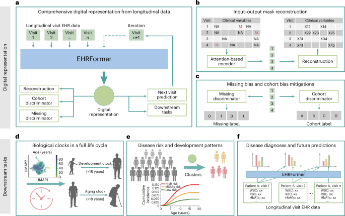
EHRFormer is an encoder–decoder style transformer architecture specifically designed to process longitudinal EHR data. The model comprises three key components: an examination encoder, a temporal embedding and task-specific decoder heads.

EHRFormer architecture and examination encoder

After preprocessing each patient’s longitudinal EHR data through discretization and concatenation into a unified feature representation as \({X}_{i}=[{X}_{{\rm{c}}{\rm{a}}{\rm{t}}};\,{X}_{{\rm{c}}{\rm{o}}{\rm{n}}{\rm{t}}}]\), we implemented a visit-level encoding framework. Similar to a BERT’s⁵⁸ embedding approach, our embedding layer employed a dual representation strategy: discretized feature values were encoded using shared token embeddings to represent their magnitude, and separate type embeddings were assigned to each variable position to denote the specific clinical feature category. This complementary embedding method allowed the model to simultaneously capture both the value distributions and the semantic meaning of different clinical measurements. A designated special vector reserved (preserved) missing examinations, enabling the model to differentiate between absent tests and actual clinical observations. To capture complex interdependencies between clinical variables, we applied a transformer-based architecture that processed these embedded features through multiple self-attention layers. This encoding process can be formalized as \({E}_{{\rm{v}}{\rm{i}}{\rm{s}}{\rm{i}}{\rm{t}}}=\text{Encoder}(\text{Embed}({X}_{i}))\), where Encoder is a Transformer encoder that generates a contextualized representation for each clinical visit.

EHRFormer architecture, temporal embedding and decoder

To model disease progression and capture the longitudinal nature of patient trajectories, we implemented a temporal embedding to capture the relative time between visits. From the examination encoder output, we retrieved a visit-level embedding, E_visit. To model temporal relationships, we used days elapsed since the initial visit as a linear positional embedding TimeEmbed (T) to enable the architecture to learn time-dependent patterns in longitudinal EHR data. To create a longitudinal patient-level representation, we passed visit embeddings E_visit augmented with time information through a Transformer decoder: E_patient = Decoder (E_visit + TimeEmbed (T)), where causal masking ensures unidirectional information flow in this autoregressive process.

EHRFormer architecture and task-specific decoders

Following the established patient-level longitudinal representation E_patient, we designed a task-specific decoder with separate pathways for discrete outcomes (for example, diagnosis prediction) and continuous measurements (for example, biomarker estimation and BA prediction). Each pathway applies a projection layer followed by ReLU activation, formalized as \({y}_{i}={\rm{R}}{\rm{e}}{\rm{L}}{\rm{U}}({W}_{i}^{{\rm{T}}}{E}_{{\rm{p}}{\rm{a}}{\rm{t}}{\rm{i}}{\rm{e}}{\rm{n}}{\rm{t}},\,i})\), where E_patient, i represents a patient’s digital representation derived from first to ith visit. Importantly, causal masking prevents information from future visits from influencing predictions at the ith visit, ensuring fairness by restricting the model to only information available in real clinical scenarios. This architecture also enables simultaneous handling of diverse clinical prediction tasks while facilitating knowledge transfer between related objectives through jointly optimized parameters.

Training procedures

Our training procedure consisted of two stages: pretraining and fine-tuning. During pretraining, we employed self-supervised learning on unlabeled longitudinal EHR data to develop robust clinical representations. The subsequent fine-tuning stage adapted these representations for specific prediction tasks. This approach leverages generalizable patterns from large-scale unlabeled data before specializing downstream applications. Both stages utilize specialized loss functions and incorporate strategies to mitigate dataset-specific biases.

Controlling for missingness and cohort bias through adversarial methods

Missing values in EHRs lead to incomplete or biased digital representations, as models may inadvertently learn to rely on the missing-state biases rather than the true clinical meaning of the feature expression values. Drawing inspiration from examples of the concept of adversarial learning in other domains, we implemented a missingness discriminator output head. Concurrently, the missingness discriminator is designed to determine whether a specific feature value is missing or not. We implemented a gradient reversal layer (GRL) between the feature encoder and the missingness discriminator. During backpropagation, the GRL inverts the gradient, compelling the feature encoder to produce representations that are independent of the missingness status. This forces the encoder to focus on encoding the inherent clinical importance of the features rather than being influenced by whether a value is present or absent. The loss function for the missingness discrimination task is defined as \({{\mathcal{L}}}_{{\rm{m}}{\rm{i}}{\rm{s}}{\rm{s}}{\rm{i}}{\rm{n}}{\rm{g}}}=-\frac{1}{M}{\sum }_{j=1}^{M}{\sum }_{m=0}^{1}z_{j,\,m}{\rm{l}}{\rm{o}}{\rm{g}}{\hat{z}}_{j,\,m}\), where \(z_{j,\,m}\) is a binary indicator denoting whether the feature value of sample j has a missing status m (0 for present, 1 for missing), \(\hat{{z}}_{j,\,m}\) is the predicted probability, and M is the number of samples with potential missing values. By minimizing this loss, the model is encouraged to learn missing-invariant representations. This approach enables the creation of more robust digital representations that can better generalize across datasets with different missing value patterns, ultimately improving the accuracy and reliability of clinical outcome predictions.

Cohort bias, also known as a batch effect, is a substantial challenge in multi-center data studies. Clinical data collected from different hospitals often exhibit systematic variations due to differences in patient demographics, practice patterns and measurement protocols, potentially leading to biased models. Similar to the missingness discriminator, we designed a cohort discriminator that aims to identify the cohort label of each sample, while the encoder is forced to suppress cohort-specific information. The cohort classification loss is formulated as \({{\mathcal{L}}}_{{\rm{c}}{\rm{o}}{\rm{h}}{\rm{o}}{\rm{r}}{\rm{t}}}=-\frac{1}{N}{\sum }_{i=1}^{N}{\sum }_{d=1}^{D}{y}_{i,\,d}{\rm{l}}{\rm{o}}{\rm{g}}(\,\hat{{y}}_{i,\,d})\), where \({y}_{i,\,d}\) is a binary indicator of whether sample i belongs to domain d, \(\hat{{y}}_{i,\,d}\) is the predicted probability, N is the number of samples, and D is the number of domains (clinical cohorts). This approach encourages the model to learn cohort-invariant representations that generalize across healthcare settings while maintaining predictive performance for clinical outcomes.

Pretraining step

We employed a self-supervised pretraining approach with multiple complementary objectives to enable our model to learn comprehensive representations of EHR data. We randomly masked 50% of the valid test results in the current examination as input, and trained the model to predict 50% masked values in the current examination and next examination. The masked language modeling loss function is defined as \({{\mathcal{L}}}_{{\rm{M}}{\rm{L}}{\rm{M}}}=\frac{1}{|{\mathcal{M}}|}{\sum }_{i=0}^{N}{\sum }_{j\in {{\mathcal{M}}}_{i}}{{\mathcal{L}}}_{{\rm{M}}{\rm{S}}{\rm{E}}}(\hat{{v}}_{i,\,j},{v}_{i,\,j})\), where \({{\mathcal{M}}}_{i}\) is the set of masked indices in examination event s_i and the next examination after s_i, \(|{\mathcal{M}}|\) is the total number of masked tokens across all examination events, v_i, j is the true value of the jth test in examination s_i and the next examination after s_i, and \(\hat{{v}}_{i,\,j}\) is the predicted value. To quantify uncertainty in the clinical data, we incorporated a variational framework with evidence lower bound (ELBO) maximization as \({{\mathcal{L}}}_{{\rm{E}}{\rm{L}}{\rm{B}}{\rm{O}}}={E}_{{q}_{\phi }}[{\rm{l}}{\rm{o}}{\rm{g}}{p}_{\theta }(x|z)]-{D}_{{\rm{K}}{\rm{L}}}({q}_{\phi }(z|x)||{p}_{\theta }(z|x))\), balancing reconstruction fidelity against latent space regularization. Additionally, we incorporated the domain adversarial loss \({{\mathcal{L}}}_{{\rm{d}}{\rm{o}}{\rm{m}}{\rm{a}}{\rm{i}}{\rm{n}}}\) and \({{\mathcal{L}}}_{{\rm{m}}{\rm{i}}{\rm{s}}{\rm{s}}{\rm{i}}{\rm{n}}{\rm{g}}}\) to promote cohort-invariant and missing-invariant representations. Finally, for the age regression task, we trained the model to predict patients’ ages at each examination event using only clinical measurements (with all age-related information explicitly removed from inputs) to assess biological aging patterns, using the mean squared error (MSE) loss function defined as \({{\mathcal{L}}}_{{\rm{a}}{\rm{g}}{\rm{e}}}=\frac{1}{N}{\sum }_{i=0}^{N}{(\hat{{a}}_{i}-{a}_{i})}^{2}\), where \(\hat{{a}}_{i}\) is the predicted age at the examination event s_i, and a_i is the true age. Only healthy individuals were included in the loss calculation for the age-prediction task, enabling EHRFormer to construct a biological clock reflecting normal aging patterns. This approach allows subsequent precise assessment of BA deviations between diseased individuals and their healthy peers in subsequent CA–BA differential analyses. Therefore, the final pretraining objective combined these components with appropriate weighting coefficients: \({{\mathcal{L}}}_{{\rm{p}}{\rm{r}}{\rm{e}}{\rm{t}}{\rm{r}}{\rm{a}}{\rm{i}}{\rm{n}}}={\alpha }_{1}{{\mathcal{L}}}_{{\rm{M}}{\rm{L}}{\rm{M}}}+{\alpha}_{2}{{\mathcal{L}}}_{{\rm{E}}{\rm{L}}{\rm{B}}{\rm{O}}}-{\alpha }_{3}{{\mathcal{L}}}_{{\rm{c}}{\rm{o}}{\rm{h}}{\rm{o}}{\rm{r}}{\rm{t}}}-{\alpha }_{4}{{\mathcal{L}}}_{{\rm{m}}{\rm{i}}{\rm{s}}{\rm{s}}{\rm{i}}{\rm{n}}{\rm{g}}}+{\alpha }_{5}{{\mathcal{L}}}_{{\rm{a}}{\rm{g}}{\rm{e}}}\), where the negative sign reflects the gradient reversal mechanism.

Fine-tuning step for disease state prediction tasks

We implemented three distinct disease prediction tasks that reflect different clinical scenarios: first occurrence disease diagnosis, future disease prediction and fixed-time-window future prediction.

For first occurrence disease diagnosis, we trained the model to identify the first occurrence of specific diseases, excluding subsequent visits after initial diagnosis to capture true onset patterns rather than disease management. Formally, for a patient with a longitudinal sequence S with length L, and where l_i, d represents whether this patient was diagnosed as positive for disease d at the ith visit, the label c_i, d of the first occurrence diagnosis task is defined as

For the future disease prediction task, we developed a labeling strategy to identify patients at risk before disease manifestation, using each visit as a dynamic baseline for prediction. Formally, for a patient with longitudinal sequence S with length L, the label f_i, d of the future prediction task for disease d at the ith visit is defined as

The third prediction task assesses N-year disease incidence. This is achieved by predicting over a fixed look-ahead window (t = 5 or 10 years) from each potential per-visit baseline. To ensure the validity of our labels, we implemented rigorous censoring for any observation with insufficient follow-up time. Formally, for a patient with recorded age A(i), the rolling t-year window prediction label \({w}_{i,\,d}^{t}\) of disease d at visit i is defined as

The loss function for each task is \({\mathcal{L}}=\frac{1}{N}{\sum}_{i=0}^{N}{\sum }_{d=1}^{D}{{\mathcal{L}}}_{{\rm{B}}{\rm{C}}{\rm{E}}}({\hat{y}}_{{i},\,{d}},\,{y}_{{i},\,{d}})\), where \(\hat{{y}}_{i,\,d}\) is the predicted probability of disease d on one of the above three labels, D is the total number of diseases considered, and \({{\mathcal{L}}}_{{\rm{B}}{\rm{C}}{\rm{E}}}\) is the binary cross-entropy loss.

Implementation details

We implemented our EHRFormer architecture using a combination of transformer models. Specifically, we utilized a 24-layer transformer encoder with a hidden dimension of 1,024 as the examination encoder to process individual examination events, and a 12-layer autoregressive transformer decoder with a hidden dimension of 768 as the temporal encoder to capture longitudinal patterns across the sequence of examinations. This design leverages the attention capabilities of the multi-headed self-attention mechanism for understanding relationships between clinical measurements within each examination, while employing the causal masked attention mechanism to model the temporal progression of patient health.

The model was implemented using PyTorch and trained using a two-stage approach. For the pretraining phase, we trained the model for 200 epochs using the Adam optimizer with a learning rate of 10⁻³ and a weight decay of 10⁻⁶. The subsequent fine-tuning phase for the downstream tasks was conducted for 100 epochs using the Adam optimizer with a reduced learning rate of 10⁻⁴, while maintaining the same weight decay of 10⁻⁶.

For both pretraining and fine-tuning steps, we utilized subsets (CHAI-Training and CHAI-Tuning) from the CHAI-Main dataset. Internal validation results were reported using CHAI-Internal, and external validation was conducted using two independent cohorts: CHAI-External-1 and UKB-External. To ensure methodological rigor, we implemented a patient-level non-overlapping partitioning strategy, randomly dividing the CHAI-Main dataset in an 8:1:1 ratio to generate the CHAI-Training, CHAI-Tuning and CHAI-Internal subsets, respectively. The healthy participants in CHAI-Main constituted the CHAI-Healthy Controls cohort used for BA calculation and age difference analysis. The UKB-External dataset comprised all available samples from the UK Biobank cohort.

Age difference calculation

To quantify biological aging deviations, we calculated standardized age differences for each individual using our aging model. First, we predicted BA A_b using the pretrained EHRFormer model on healthy participants in CHAI-Healthy Controls. We then modeled the nonlinear relationship between predicted BA A_b and CA A_c using locally weighted scatterplot smoothing (LOWESS) with a bandwidth parameter of 2/3 via the statsmodels Python package (version 0.14.4) using EHR data from healthy individuals. The resulting function f(A_c) represents the expected BA for a given CA based on healthy population trends. For each individual i, we calculated the raw age difference as \({{\varDelta}}_{i}={A}_{{b},\,{i}}-f({A}_{{c},\,{i}})\), representing a deviation from healthy peers with the same CA. Finally, we computed standardized age differences as \({z}_{i}={{\varDelta}}_{i}/\sigma\), where σ represents the s.d. of raw age differences within the model.

Visualization of latent space and disease risk analysis

Visualization and clustering of EHRFormer-derived latent vectors were performed by first extracting the laboratory and vital sign features, followed by PCA with 50 components. The resulting embeddings were processed using a neighbor graph approach (15 neighbors, Euclidean metric) and visualized with UMAP (parameters: min_dist=0.3, spread=1.0, 2 components, spectral initialization). Cluster identification was performed using the Leiden community detection algorithm, revealing distinct patient groups that correspond predominantly to pediatric and adult populations. For disease visualization, prevalence and incidence proportions were calculated per cluster. Prevalence was defined as the proportion of individuals with pre-existing disease at baseline (first hospital encounter). Incidence was calculated as the proportion of initially disease-free individuals who developed the condition during the follow-up period (five years from first admission). Each data point was colored according to its corresponding cluster-specific disease prevalence or incidence proportion, providing a visual representation of disease burden across identified patient subgroups. PCA, UMAP and projection visualizations were constructed using the Scanpy⁵⁹ Python package (version 1.10.4).

Disease–cluster associations were quantified using adjusted log₂HRs, calculated for each cluster based on the cluster of each patient at their first clinical visit in reference to the remainder of the study population using Cox proportional hazards models. These models incorporated multivariate adjustment for patient demographics (age and sex), smoking, alcohol history and hospital to minimize potential confounding. These associations were visualized using a heatmap with log₂HR values truncated at a maximum of 2 to enhance interpretability while preserving meaningful signal contrast. HRs were calculated using the lifelines Python package (version 0.30.0).

Statistical analysis

We evaluated the performance of regression models for continuous value predictions using MAE, R² and PCC. Binary classification models were evaluated using receiver operating characteristic (ROC) curves showing sensitivity versus 1–specificity, with the AUC reported along with 95% confidence intervals. AUCs were calculated using the scikit-learn package (version 1.6.1). Cumulative incidence curves for deciles of disease risk score were calculated using KaplanMeierFitter from the lifelines Python package (version 0.30.0). We plotted cumulative events against each visit age on the x axis. Incidence rates for subsequent records after each given visit age are shown on the y axis.

Reporting Summary

Further information on research design is available in the Nature Portfolio Reporting Summary linked to this Article.