A pangenome and pantranscriptome of hexaploid oat
DNA extraction
Plant growth and isolation of high-molecular-weight DNA
High-molecular-weight (HMW) DNA was extracted from young leaf tissue from a single two-week-old seedling grown in an isolated growth chamber under a 12-h photoperiod. The growing temperatures ranged from 18 °C (night) to 20 °C (day). The hydroponic growth solution was prepared using MaxiBloom Hydroponics Plant Food (General Hydroponics) at a concentration of 1.7 g l−1. In preparation for PacBio HiFi sequencing, HMW DNA was extracted from 72-h dark-treated leaf samples using a CTAB-Qiagen Genomic-tip protocol as described previously42. DNA quantification and purity were checked using a Qubit dsDNA HS assay and a NanoDrop spectrophotometer, respectively.
Short-read sequencing
Six assemblies included in PanOat have already been published: A. insularis (BYU209), A. longiglumis (CN58138) and Sang4; A atlantica and A. eriantha15; and OT3098, which was made available as a free resource by PepsiCo in 2020 and was later improved to pseudomolecules (https://wheat.pw.usda.gov/GG3/graingenes-downloads/pepsico-oat-ot3098-v2-files-2021, PRJEB76239 and PRJEB46951).
The A. byzantina PI258586 contig assembly was assembled using the TRITEX43 pipeline and Hi-C data from the Dovetail Omni-C platform. Genome assemblies for Gehl and AC Nicolas were scaffolded using TRITEX and Hi-C to guide pseudomolecule assembly43.
PacBio HiFi sequencing
DNA library preparation and PacBio HiFi sequencing
HMW genomic DNA was sheared to 17 kb on a Diagenode Megaruptor and then converted into SMRTbell adapted libraries using SMRTbell Express Template Prep Kit 2.0. Size selection was performed using a Sage Blue Pippin to select fragments greater than 10 kb. These were then sequenced at the Brigham Young University (BYU) DNA Sequencing Center, except for the ‘Aslak’ accession, which was sequenced at the DNA Sequencing and Genomics Laboratory, Institute of Biotechnology, University of Helsinki, using the Sequel II Sequencing Kit 2.0 with Sequencing Primer v.5 and Sequel Binding kit 2.2. Run times were 30 h with adaptive loading, following PacBio SMRT Link recommendations.
Hi-C sequencing
In situ Hi-C libraries were prepared from young seedlings according to the previously published protocol, using DpnII for the digestion of cross-linked chromatin2 or with a Phase Genomics multi-enzyme mix. Sequencing and Hi-C raw data processing were performed as previously described44.
Genome sequence assembly and validation
Chromosome-scale assembly
TRITEX + Dovetail Omni-C
Chromosome-scale sequence assembly proceeded in three steps: (i) scaffold assembly using the TRITEX pipeline45; (ii) super-scaffolding with the Dovetail HiRise pipeline46 (v.2.0.5) using Omni-C data; and (iii) arranging super-scaffolds into chromosomal pseudomolecules using TRITEX (https://tritexassembly.bitbucket.io). PE450 reads were merged with BBmerge47, error-corrected with BFC48 and assembled with Minia349. Scaffolding and gap filling were done with SOAPDenovo250 using MP6 and MP9 data. Super-scaffolds were generated with the Dovetail HiRise pipeline (v.2.0.5) from alignments of Omni-C data to scaffolds. Omni-C reads were aligned to the HiRise super-scaffolds with Minimap251. Alignment records were converted to binary Sequence Alignment/Map format using SAMtools52 and sorted with Novosort (http://www.novocraft.com/products/novosort/). A list of Omni-C links was extracted from Hi-C alignments using TRITEX scripts. Omni-C links and guide-map alignments were imported to the R statistical environment53 and analysed further using TRITEX scripts. An initial Hi-C map was generated using the minimum spanning tree algorithm described previously54. The assembly and Hi-C map were iteratively corrected by inspecting Hi-C contact matrices, guide-map alignments and physical-coverage Hi-C reads. Sequence files in FASTA format and AGP tables for pseudomolecules were compiled using TRITEX scripts. The pseudomolecules of A. byzantina were aligned against the pseudomolecules constructed from a long-read sequence assembly of cv. OT3098. The OT3098 pseudomolecules (v.2)8 were downloaded from GrainGenes55.
PacBio HiFi
PacBio HiFi reads were assembled using hifiasm (v.0.14.1)56 and the TRITEX pipeline45 was used for pseudomolecule construction. Chimeric contigs and orientation errors were identified through manual inspection of Hi-C contact matrices43. GMI423 was used as the reference to map HiFi contigs, using a reduced single-copy genome.
Note on chromosome 7D: while assembling chromosome 7D, we noticed that, when aligning several of our genotypes to GMI423, there was a large, approximately 450-Mb inversion and a small approximately 50-Mb sequence with the same orientation as GMI423. We decided to flip the long sequence to the same orientation as GMI423 and flip the small sequence to the inverted orientation, thinking that the small segment was translocated from one end of the chromosome to the other. Retrospectively, this was a mistake. The more plausible explanation would be an inversion of the large sequence, as supported by several genetic studies57 showing a distinct lack of recombination in this region.
Multidimensional scaling (MDS) of Global Oat Diversity GBS data
A total of 9,111 lines from the Global Oat Diversity (G.O.D.) collection14 were analysed together with the PanOat assemblies. All of the GBS sequencing data from the G.O.D. lines were aligned to a single reference genome (GS7) using BWA followed by sorting using NovoSort and indexing with SAMtools. The PanOat assemblies were aligned to the GS7 genome. We simulated short reads (tenfold coverage) using the fastq generator (https://github.com/johanzi/fastq_generator) and mapped these to GS7 using Minimap251, followed by sorting using NovoSort and indexing with SAMtools. The resulting mapping files from the PanOat assemblies and the G.O.D. were merged into a VCF file using bcftools mpileup58 with filtering for Q40 or larger and a minimum of 50% missing data per position or SNP.
MDS analysis was preformed using PLINK59 (www.cog-genomics.org/plink/1.9/) with –maf=0.05 and a maximum of 70% missing data. Results were plotted in R using the ggplot2 package.
Single-copy pangenome
A single-copy pangenome was constructed as described previously60 (https://bitbucket.org/ipk_dg_public/barley_pangenome/), with one modification. MMSeq261 was used with the option ‘ –cluster-mode’ instead of BLAST for all-versus-all alignment. A minimum sequence identity of 95% was required to accept matches. To estimate the pangenome size, the lengths of the largest sequences in each cluster were summed up.
PanOat transcriptome sequencing
Plant materials, growing conditions and tissue dissection
A subset of 23 PanOat genotypes was selected for transcriptome sequencing (Supplementary Table 2). RNA was extracted from six tissues (Extended Data Fig. 2a–c and Fig. 2a). The 23 genotypes were grown in 6 sets for sampling each tissue separately. Each set comprised at least nine biological replicates (different plants) per oat genotype. Every set with replicates was grown in a separate unit of the growth facility and allocated randomly using the ‘sample’ function in the R statistical environment62. Sampled tissues from 3 different plants (3 technical replicates) were pooled into one tube, making one biological replicate, and this process was repeated twice more to collect a total of 3 biological replicates for each of the 23 PanOat genotypes chosen and the 6 selected tissues (Extended Data Fig. 2a–c).
Embryonic tissues
Seeds were sterilized in ethanol (70%) and sodium hypochlorite (50%), then rinsed five times in sterile water, followed by germination of dehulled seeds in Petri dishes (50 mm; covered in two layers of aluminium foil to maintain darkness) in a growth chamber under constant temperature (about 18 °C), humidity (about 75% relative humidity) and 16-h days. Parts of the coleoptile, mesocotyl and seminal roots were dissected from germinating seeds starting from four days after germination (Extended Data Fig. 2b). These were promptly frozen in liquid nitrogen and stored at −80 °C and thawed before RNA extraction.
Leaf tissue
Seedlings were germinated from sterilized seeds as above, but larger Petri dishes (120 mm) were used. Seedlings were grown until two leaves had emerged. Then, the middle part of the leaf blade was dissected for RNA extraction.
Root tissue
Seedlings were grown in a small pot on a perlite substrate until three leaves had emerged (Extended Data Fig. 2b). Roots were then separated from the perlite and rinsed in sterile water. Cleaned roots were dissected from the top parts of the plants and stored at −80 °C until RNA extraction.
Stem tissue
Plants were grown in pots (one seed per pot) on a soil substrate in a greenhouse chamber with constant temperature (20 °C) and semi-controlled light conditions (16-h light period) until the main stem and four tillers had developed (Extended Data Fig. 2b). Two-millimetre-wide stem discs were dissected from the internode elongating below the flag leaf.
Panicle tissue
Plants were grown as above until the main stem and five tillers had developed (Extended Data Fig. 2b). A developing panicle with a size not longer than 15 mm was dissected from the main tiller.
Caryopsis tissue
Plants were grown as above until the phenophase in between kernel water ripe with no starch and early milk (Extended Data Fig. 2a,b). This phenophase is recognized to happen four days after anthesis63.
RNA extraction
Total RNA from embryo tissues, leaves, roots, stem and developing panicle was extracted using the RNeasy Plant Mini Kit (QIAGEN). Total RNA from developing caryopsis tissues was extracted using the RNeasy PowerPlant Kit (QIAGEN), according to the manufacturer’s instructions. Before RNA extraction, all samples were digested using RNase-free DNase (QIAGEN). Tissue samples were thawed and processed in a random order. Extracted RNA was diluted in 100 μl of buffer and checked for degradation, quantity and purity. RNA integrity was checked using an Agilent Bioanalyzer. Purity (absence of contaminating proteins) was checked by measuring the fluorescence absorbance of nucleic acids at 260 nm and 280 nm using a NanoDrop spectrophotometer. RNA amounts were determined using a Qubit fluorometer (Thermo Fisher Scientific). Average RNA integrity numbers (RINs) varied from 7.62 in leaf tissues to 9.50 in developing panicles and stem tissues. RIN was, on average, lower in leaf tissues but varied little between samples. Only pure RNA samples with high RIN scores (greater than 8.5, except leaves) and sufficient concentration were used for further processing.
Illumina RNA-seq
Sequencing libraries were prepared for 432 high quality total RNA samples (RIN > 7.62). First, 500–1,000 ng of total RNA were Poly(A+) enriched, then RNA-seq libraries were produced using the CORALL mRNASeq V1 kit according to the manufacturer’s instructions (Lexogen) For each library, barcoding was done using unique dual indices (UDI). To avoid any experimenter’s bias, the preparation of the libraries was done randomly. Sequencing was done in 8 pools, with each pool containing 54 randomized single libraries in equimolar amounts. Before sending the pools to the sequencing facility, each pool was sequenced on the iSeq 100 benchtop sequencer at the Natural Resources Institute Finland (LUKE) for quality control. Paired-end sequencing (2 × 150 bp) was done on a Novaseq 6000 device (Illumina) distributed on two full S4 flow cells at the Finnish Functional Genomics Centre in Turku, Finland. Sequencing (2 × 150 bp) of nine libraries was repeated on a NextSeq 550 device (Illumina) in the genomics laboratory at LUKE. The total number of raw reads per sample and the BioSample IDs are provided in Supplementary Table 17.
PacBio Iso-Seq
For each genotype, total RNAs from all tissues and replicates from the respective genotypes were pooled, with between 1,623 ng and 2,001 ng of pooled RNA used for each library. In total, 24 full-length cDNAs were prepared using the TeloPrime Full-Length cDNA kit (Lexogen). Different from the manufacturer’s protocol, the purification of 100 µl of cDNA was done with 86 µl ProNex beads (Promega), the standard size selection was done according to the Iso-SeqTM Express Template preparation protocol (PacBio) and no enrichment for shorter or longer transcripts was used. Owing to the 5′ cap specificity of this method, only full-length, double stranded cDNA was obtained. The cDNAs ranged in size from 1,000 to 5,800 bp, with mean peak values between 1,845 bp in HiFi and 2,832 bp in GMI423. After purification, the cDNAs were quantified with Qubit (Thermo Fisher Scientific). According to the Iso-Seq Express Template preparation protocol (PacBio) the amount of cDNA should be in the range of 160–500 ng for Sequel II systems. Libraries with a lower amount of cDNA were re-amplified following the PacBio guidelines. After DNA damage repair, end repair, A-tailing, overhang adapter ligation and clean up, the concentrations were checked using Qubit. The quality was verified using a Bioanalyzer (Agilent). Twenty-four cDNA SMRTbell libraries with a mean fragment length distribution between 2,155 bp and 3,557 bp were transferred to the sequencing facility. The Iso-Seq SMRTbell libraries were sequenced at BYU, each library in a separate Sequel II run. Numbers of reads and total read lengths are provided in Supplementary Table 1.
Annotation of protein-coding genes
For the 23 oat lines with native transcriptome data generated in this study (Supplementary Table 2), we performed de novo structural gene prediction, confidence classification and functional annotation, following a protocol described previously17. The strategy applied in this study differs only in the use of TE soft-masked genome sequences instead of TE hints (see ‘Repeat-masking for gene detection’). We applied the same gene prediction procedure for the de novo annotation of the lines A. sterilis TN4 and A. byzantina PI258586 using transcriptome data as evidence. Gene predictions for the lines OT380, A. sterilis TN1, A. fatua CN25955, A. eriantha BYU132/CN19328 and A. atlantica Cc7277, which had no native transcriptome data, were done using a gene consolidation approach that has been described previously16. Here, the gene predictions for all 30 oat lines described above were cross-mapped with the genome sequences of one another to identify and correct for missed gene models and to annotate genomes without native transcriptome data.
Finally, for the three lines Leggett, Williams and AC Morgan, we predicted their gene content using the projections of the aforementioned evidence-based gene models to their genomic sequences. The principle of the projection method is described in https://github.com/GeorgHaberer/gene_projection; applied parameters of the workflow and code have been deposited in the directory ‘panoat’ in the parent directory.
Repeat-masking for gene detection
To minimize the inclusion of transposon-related gene models, the genome assemblies were soft-masked for transposons (TEs) before gene detection. The TE library used, developed for the oat reference genome4, masked approximately 60% of the assembly for each line. Soft-masking was performed using vmatch (anaconda.org/bioconda/vmatch, v2.3.0) with the following parameters: ‘-l 75 -identity 70 -seedlength 12 -exdrop 5 -d -p -qmaskmatch tolower’.
Construction of the oat core, shell and cloud genomes
Phylogenetic HOGs based on the primary protein sequences from 30 oat lines with consolidated gene predictions were calculated using OrthoFinder v.2.5.520 with standard parameters (see ‘Annotation of protein-coding genes’ for details; Leggett, Williams and AC Morgan were not part of this orthologous framework, because their gene content was not consolidated). Before the analysis, input sequences were filtered for transposon- and plastid-related proteins and proteins encoded on unanchored contigs were discarded for this analysis.
Depending on the focus of the analyses, we treated each of the subgenomes of hexaploid and tetraploid oat lines either as individual entities or, for our analysis of core, shell and cloud genomes, as parts of the single lines.
The scripts for calculating core, shell and cloud genes have been deposited in the repository https://github.com/PGSB-HMGU/BPGv2.
Core HOGs contain at least one gene model from all 30 compared oat lines. Shell HOGs contain gene models from at least 2 oat lines and at most 29 oat lines. Genes that were not included in any HOG (singletons), or were clustered with genes only from the same line, were defined as cloud genes.
GENESPACE64 was used to determine syntenic relationships between the chromosomes of all 30 oat lines.
Protein functional annotation and gene-set enrichment analysis
For functional enrichment analysis in the identified expression level categories, Mercator465 (v.6.0) protein functional annotation was performed for the identified 5,291 single-copy HOGs across the 20 A. sativa lines, which yielded 4,682 protein annotations (Supplementary Table 18). These annotations were used to test enrichment using over-representation analysis (ORA) of sets of genes associated with expression level categories with the R package clusterProfiler66 (v.4.6) and a Benjamini–Hochberg FDR correction P value cut-off of 0.05.
Similarly, for ORAs across genes classified into core, shell and cloud categories, all of the 31 oat lines’ proteomes (2,869,876 proteins and 131,729 HOGs) were functionally annotated with Mercator4 (v.6.0). This resulted in a total of 53,018 annotated HOGs for the core (8,325 annotated HOGs), shell (32,108 annotated HOGs) and cloud (12,585 annotated HOGs) categories, applied as universe in the enrichment analyses. ORAs showed enrichment across multiple Mercator4 hierarchical categories (labelled as levels 1–7) (https://hmgubox2.helmholtz-muenchen.de/index.php/s/Y3wWa7bn2rayEqw).
Gene-expression analyses
For the analysis of gene expression, RNA-seq data from 23 oat varieties (Supplementary Table 2) were processed using Fastp67 (v.0.24.1) for trimming, followed by quality assessment and outlier detection. The data for each line were aligned to the relevant reference genome using Kallisto68 (v.0.48; Supplementary Figs. 2 and 3) and normalized to transcripts per million (TPMs) using Deseq2’s tximport function69,70. All RNA-seq data were also aligned to the GS7 reference genome for specific analyses.
To compare the expression levels across different subgenomes (A, C and D), gene-expression data from six tissues (leaf, embryo, root, internode, panicle and caryopsis) were examined.
We focused on high-confidence genes and for each gene, the expression value was normalized using a log transformation (log(value + 1)) to stabilize variance and ensure that the data were suitable for statistical comparisons. The log-transformed expression values were aggregated by calculating the mean expression level for each line, tissue and subgenome combination. To determine whether the expression levels between different subgenomes were significantly different, Mann–Whitney U tests were performed for each tissue type. Comparisons were made between each pair of subgenomes (A versus C; A versus D; and C versus D).
For the purpose of identifying genes with stable versus variable expression, the analysis was limited to 20 A. sativa varieties and 5,965 HOGs. These HOGs were characterized as single-copy orthologues with an A:C:D ratio of 1:1:1 across all 20 varieties, providing a standardized basis for comparison. HOGs were deemed stable if 90% of the varieties exhibited the same expression category; otherwise, they were classified as variable.
In the set of 5,965 ‘60-lets’, expression levels were categorized into one of 7 categories on the basis of the Euclidean distance to 7 ideal expression level profiles: A-, C- or D-dominant or A-, C- or D-suppressed, in which one gene is predominantly expressed or suppressed, and a balanced category, in which A, C, and D genes are equally expressed, as outlined previously4.
Analysis of differences in gene expression between diads and triads
We focused on the 20 A. sativa lines and selected genes that had either one single-copy homeologue in each of the subgenomes (so forming complete triads: A:C:D 1:1:1 constitution) or a constitution in which one triad member was missing (so forming diads: A:C:D 1:0:1, 1:1:0 or 0:1:1). The lines were then categorized into groups with complete triads and diads, while ensuring uniformity in the missing pattern across the lines. This approach allowed for a controlled comparison across genetic backgrounds. To ensure robust statistical analysis, specific filtering criteria were applied. Each group analysed was required to consist of at least five lines, allowing us to achieve sufficient statistical power.
We used an unpaired t-test to assess the significance of expression differences between groups with a missing homeologue and those with complete triads. Furthermore, Cohen’s d was used to determine the directionality of these differences. A chi-squared test was used to compare the frequency of significant compensatory expressions across the different subgenomes.
Analysis of changes in gene expression at translocation break points
To assess gene-expression changes associated with translocation break points, we first identified the break points on the basis of the GS7 genome by aligning the chromosomes of each oat line to GS7 using Minimap251. We then extracted 100 syntelogues on either side of each break point using GENESPACE64.
For gene-expression profiling, RNA-seq data from all oat lines were mapped to the GS7 transcriptome using Kallisto68, and differential gene-expression analysis was performed with DESeq269. Gene expression was compared across multiple tissues between lines carrying each translocation and those without.
To determine whether the regions surrounding translocation break points were significantly enriched for differentially expressed genes relative to the rest of the chromosome, we applied a hypergeometric test. This statistical test assesses whether the observed number of DEGs in the translocation regions exceeds what would be expected by chance, given the total number of genes and DEGs on the chromosome. Statistical significance was determined using an FDR-adjusted P value (Benjamini–Hochberg correction, α = 0.05).
Comparative gene-expression analysis in ND060432
Total RNA was extracted from young leaf blades of ND060432 in four biological replicates and sequenced using the same protocol as was used for the other PanOat leaf samples. RNA-seq reads from the leaf samples of GS7 and ND060432 were processed with Fastp67 (v.0.24.1) for trimming and quality assessment. Processed reads were aligned to the GS7 reference transcriptome using Kallisto68 (v.0.51.1) and normalized to TPMs. Expression values of biological replicates were summarized to their median value. To investigate whether the substitution of chromosome 6D with 6A affects gene expression, we compared the expression ratio of A- to D-subgenome genes within each chromosome group, with a particular focus on changes on chromosome 6D. Each chromosome was divided into 20 bins that were proportional in size to the size of the chromosomes. The expression was then summarized to the average value per bin. Statistical comparisons were performed using the Wilcoxon rank-sum test with FDR correction for multiple comparisons in the seven chromosome pairs. Significance levels were denoted as: ***P < 0.001, **P < 0.01, *P < 0.05, NS, not significant. Effect size was calculated as r = |Z | /√N, where Z is the standardized test statistic and N is the total sample size (n = 40 per comparison: 20 bins per chromosome × 2 chromosomes; Supplementary Table 16).
To further study the effect of the replacement of chromosome 6D with chromosome 6A in ND060432, subgenome expression bias categories were quantified. Therefore, triads were identified in each of GS7 and ND060432. Expression levels of triads overall and in each chromosome group were categorized into one of seven categories on the basis of the Euclidean distance to seven ideal expression level profiles: A-, C- or D-dominant or A-, C- or D- suppressed, in which one gene is predominantly expressed or suppressed, and a balanced category, in which A, C and D genes are equally expressed, as outlined in a previous study4. Because oat has many translocations and triad genes can be located on chromosomes of different chromosome groups, triad membership to a certain chromosome group was determined according to the location of the D-subgenome gene to investigate the effect of the replacement of chromosome D. In addition, ternary plots were generated to visualize these subgenome expression patterns across all triads and within chromosome groups 1–7. These plots illustrate the distribution of expression bias among the three subgenomes, where points near the vertices indicate subgenome-specific dominance and points near the centre represent balanced expression. Statistical significance of the bias in the patterns was assessed using chi-squared tests for each chromosome group (Supplementary Table 16).
WGS of the North American spring oat collection
Sequencing, mapping and GWAS of CORE samples
A total of 295 North American spring oat accessions from the CORE population32 (Supplementary Table 13) were sequenced using an Illumina Novaseq 6000 (paired-end 150 bp) with a mean read depth of 4.58 per accession.
The genome assembly of GS7 was chosen as a reference because it is a North American variety with a long-read assembly. The adapter sequence (‘AGATCGGAAGAGC’) was removed using cutadapt71 and then all reads were aligned to the GS7 reference genome using Minimap251, sorted with NovoSort (https://www.novocraft.com/products/novosort/) and converted to a compressed reference-oriented alignment map (CRAM72) file using SAMtools58. A VCF file was created using bcftools ‘mpileup’58, including all variations with mapping quality higher than 40. Read-depth variation was determined by counting how many reads were aligned in 1-Mb windows along the genome.
For GWAS, a k-mer-based reference-free pipeline was used (kmerGWAS)73. The phenotypes used included heading date, plant height and grain yield, collected from ten locations in two consecutive years (2010 and 2011 (ref. 32); Supplementary Fig. 4). k-mers with significant association (−log10 threshold for 10% family-wise error rate) were mapped to the GS7 genome.
PanOat assemblies
To align the PanOat assemblies to the GS7 genome, we simulated short reads (tenfold coverage) using fastq generator (https://github.com/johanzi/fastq_generator) and mapped these to GS7 using Minimap251. The resulting mapping files were merged into a VCF file together with all 295 CORE genotypes using bcftools merge58.
Genome alignments
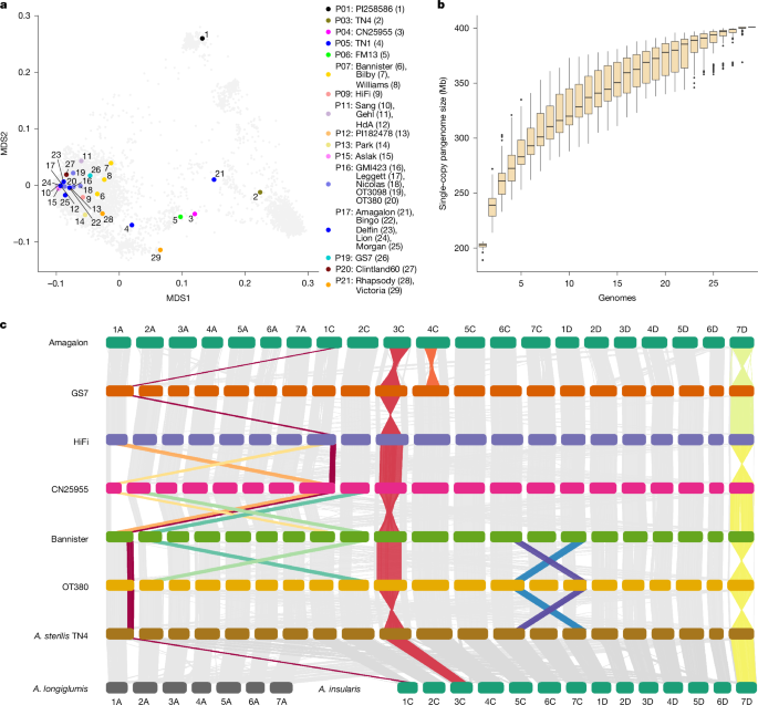
Whole-genome alignments of complete pseudomolecule assemblies were performed using Minimap274 with the -f 0.05 option to filter out repetitive minimizers and speed the alignment process. Visualization was done using NGenomeSyn41 as shown in Fig. 1c.
PCA of WGS data
Focusing only on SNPs on chromosome 7D, PCA analysis was done with all 295 genotypes and PanOat assemblies using PLINK with –maf=0.05 and a maximum of 70% missing data. SNP haplotypes were analysed using a custom Perl script75 (https://github.com/guoyu-meng/barley-haplotype-script/tree/main/05.other/SNP_haplotype_plot), then sorted by the predicted inversion state from the PCA analysis and plotted in R.
Reciprocal translocation 2A/2C in Australian and Canadian oat
Plant materials
The oat varieties used in this study were part of a worldwide oat germplasm collection from the Western Crop Genetics Alliance at Murdoch University (Supplementary Table 14), and included 564 lines from 41 countries. To track down the pedigree of the chromosome 2A/2C translocation, potential parental lines for the varieties with the translocation were collected for the second-round test with 32 varieties (Supplementary Table 15.2). Seeds of the oats were grown in pots in a glasshouse, with natural lighting cycles and regular watering. Leaves from three-week-old seedlings were collected for DNA extraction.
A RIL population was derived from Bannister × Williams crossing. An F5 population was grown in the greenhouse at InterGrain. A total of 188 lines, together with their parents, were used for molecular map construction using DArTseq technology, following the online instruction (Diversity Arrays Technology). Three to five centimetres of leaf sections were collected for DNA extraction from seedlings at the three-week stage.
Chromosome-specific molecular markers for 2A/2C translocation
Genomic DNA was extracted from the leaves of each oat line using the cetyl trimethyl ammonium bromide (CTAB) method76. DNA quality was assessed on 1% agarose gels and quantified using a NanoDrop spectrophotometer (Thermo Fisher Scientific). DNA was diluted to 50 ng µl−1 for PCR.
Two DNA samples (OT207 and Kanota) used in this study were obtained from Agriculture & Agri-Food Canada, owing to the unavailability of these varieties in Australia. Specific primers for PCR (Supplementary Table 15.1) were based on sequences from the Australian oat Bannister and the Spanish oat FM13. Primers Ban2A_F3 and Ban2A_R3 are specific to the Bannister chromosome 2A break point, producing a PCR amplicon of 397 bp. Another pair of primers, Ban2C_F3 and Ban2C_R3, is specific to the Bannister chromosome 2C break point, producing a PCR amplicon of 595 bp. PCR was done in 10-µl reactions in 384-well PCR plates (Axygen) containing 50 µM of each of the three primers, 200 µM dNTPs, 1.5 mM MgCl2 and BIOTAQ (Bioline Australia) in a Veriti Thermo cycling machine. The PCR products were separated and visualized on 2% agarose gels stained with GelGreen (Biotium). Oat lines containing the 2A/2C translocation produced bands and were scored as ‘present’, whereas normal oat lines did not produce bands and were scored as ‘absent’.
Genetic map construction
The RIL lines were genotyped with DArTseq markers. The genotypes were filtered with the following parameters: call rate higher than 90%, polymorphic information content higher than 0.2 and heterozygous frequency less than 0.6. MSTmap77 (https://github.com/ucrbioinfo/MSTmap) was used to construct the genetic map77. Several rounds of calculations were performed to correct and impute genotype calls. After the first round of genetic map construction, the markers were sorted on the basis of the genetic map and considering the physical orders. Missing data and noisy markers were corrected if the physical and genetic orders were consistent. The heterozygous regions were fixed first, and then the nearby markers were corrected in subsequent rounds of calculation. The final genetic map was calculated after three to four rounds of corrections. The chromosomal 2A/2C translocation-specific molecular markers were manually integrated into the molecular linkage map.
Validation of chromosome 2A/2C fragment deletion in the RIL population of Bannister/Williams
The whole-genome DarT seq method identified ten RILs with potential chromosome fragment deletions (Supplementary Table 15.3), but only three RILs had set seeds. On the basis of DArT marker sequences, PCR primers for different locations on chromosome 2A or 2C were designed to validate the truncations seen using agarose-gel-based methods. The primer sequences and locations (aligned FM13 genome sequences) are listed in Supplementary Table 15.4. Each pair of primer sequences or a marker is unique and only has one specific amplicon.
PCR and gel analysis was performed as described above. With this set of primers, a score of ‘present’ indicated that the DNA sequence at a particular locus was normal. Those scored as ‘absent’ indicated mismatches with the primers, or that a sequence was missing. When a few consecutive loci on the same chromosome are all scored as absent, it is most likely that the section of the chromosome has been replaced or is truncated.
Sixteen markers scattered across chromosomes 2A and 2C were tested in three lines (BW041, BW080 and BW123). The three or four plants from each pot were verified to have the same genetic background. BW041 and BW080 are likely to be truncated on 2C from 412,337 kb. The tip of chromosome 2A from BW123 is missing; the truncation point is likely to be between 2A 26,716 kb and 344,891 kb. The deleted fragments were further validated by 10x whole-genome shotgun sequencing.
Yield evaluation
Grain yield data were obtained from the Australian NVT from 2018 to 2022. Each year included 19 to 31 trials across Australia, with 158 trials designed in 3 replications. There were six 2A/2C translocated varieties and 11 non-translocated varieties.
NVT is an Australian national program that provides field-collected information comparing yield performance and grain quality on commercially available grain varieties, including barley, wheat and oat. Detailed trial locations are in the oat-growing areas across the whole continent (Grains Research and Development Corporation, https://nvt.grdc.com.au). Trials follow a standard protocol to facilitate yield evaluation and comparison (https://nvt.grdc.com.au/__data/assets/pdf_file/0023/613166/NVT-PROTOCOLS-v2.0.1_FINAL.pdf).
Trial designs use statistical methodology and allow for site and subsequent across-site analysis. Trial sites were located throughout the Australian grain-growing region. Each trial had four to eight repeated cultivar entries yearly to allow connectivity among trials. Each cultivar entry was replicated in three randomly placed plots. Plot size was standard at 1.2 m by 6 m. Seed sowing and trial management followed the best local agronomic practice. Each trial was harvested at the earliest opportunity after physiological maturity to minimize grain losses through wind, insect, rain or pest damage. The field plot yield was calculated from the harvested grain. Grain yield was adjusted with linear mixed models, in which variance parameters in the mixed models were estimated using the residual (restricted) maximum likelihood (REML) procedure with ASReml-R (v.4.1.0; https://asreml.kb.vsni.co.uk/wp-content/uploads/sites/3/2018/07/ASReml-Package.pdf). Spatial variations were examined, including local autocorrelations, global trends and extraneous variations. The blocking structure of the experiments was fitted as random effects. Spatial trends and residual variances with two-dimensional auto-regressive correlation at first order for rows and columns were examined and fitted when they were statistically significant. Statistical tests were used to examine the levels of significance, including likelihood ratio tests for random effects, and conditional Wald tests for fixed effects. Residual diagnostics were performed to examine the validity of the model assumption of independence, normality and homogeneity of variance. Both the empirical best linear unbiased predictions (eBLUPs) estimated means for varieties, with variety fitted as random effects, and the empirical best linear unbiased estimations (eBLUEs) estimated means for varieties, with variety fitted as fixed effects, were produced from respective fitted models. Trials with an average grain yield of less than 1,000 kg ha−1 were deemed as abnormal and removed from further analysis.
To account for variability between trials and years, we recalculated the variety yield as the ratio to the average yield of all varieties (17) within the trial, following:
Variety yield (relative to site average) = Variety trial yield/average yield within the trial
The average variety yield (relative to site average) within a trial of translocated and non-translocated varieties across all trials was compared using a two-sided t-test with SPSS v.29 (IBM). Significance was taken as P < 0.05.
Because yield advantages are known to be associated with reduced plant height, we also examined the height of varieties with or without the 2A/2C translocation. In a common-garden experiment, the oat varieties were grown in South Perth (Western Australia) for three years. The height was measured from the tip of the panicle to the ground (detailed experiment and results are to be published in a separate paper). To account for variability between years, we calculated the height as the ratio to the average height of all (17) varieties. The height (relative to the site average) of translocated and non-translocated varieties across all trials was then compared using a two-sided t-test with SPSS v.29 (IBM). Significance was taken as P < 0.05.
QTL mapping
Plant height was measured before grain harvest. The genotypic and quantitative trait data were formatted for use with MapQTL5.0. A permutation test was performed to calculate the logarithm of the odds (LOD) value threshold for positive QTL detection. Internal mapping was first performed to identify the markers with the highest LOD value above 3.2. The markers with the highest LOD values from different QTLs were selected for multiple QTL mapping analysis.
Large-scale chromosomal rearrangements shaped segregation and recombination patterns in progenies of 13 crosses from a working oat breeding program
Thirteen F1 crosses were made in 2019 at the oat breeding program at the Ottawa Research and Development Centre, Agriculture and Agri-Food Canada (AAFC) (Supplementary Table 19.1), among oat lines that were selected for their excellent trait profiles and adaptation to Canadian environments. Progenies were advanced by a modified single-seed descent method to the F6 generation. Parents and progeny were genotyped using a targeted GBS method78. Progenies were filtered to remove those with more than 90% similarity to a parent and to eliminate progeny that showed more than 98.5% similarity to another progeny. The position of tag-level haplotype markers on the Sang reference genome4 was used to compute recombination fractions (r) between all pairs of markers. Values of r were averaged within a sliding window of 20 Mb at 10-Mb increments in two directions of a complete genome matrix, as described previously31, such that recombination fractions were scaled to physical distance. Recombination matrices across the full genome were displayed as heat maps, coloured from yellow (r = 0) to cyan (r = 0.2) to purple (r > =0.4) (also in Supplementary Table 19.2). Chromosomes with inadequate marker coverage to estimate recombination were coloured grey.
C-banding
All karyotypes of lines throughout the manuscript were determined by C-banding as described previously79, except that 0.1% colchicine at 20 °C for three to five hours was used to arrest microtubule assembly.
Reporting summary
Further information on research design is available in the Nature Portfolio Reporting Summary linked to this article.
First Appeared on
Source link

