Clinical-grade autonomous cytopathology through whole-slide edge tomography

Whole-slide edge tomography

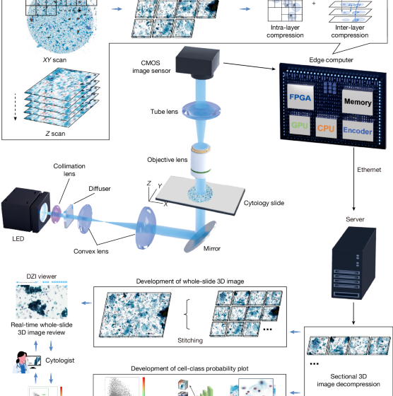
As shown in Extended Data Fig. 1, the whole-slide edge tomograph comprises multiple hardware modules optimized for high-speed 3D imaging and edge-side data processing. The illumination system uses a high-power light-emitting diode (XQ-E; Cree) as the light source, paired with a motorized iris (Nihon Seimitsu Sokki) to control the numerical aperture. This illumination passes through the cytology sample and is projected onto a camera board equipped with a CMOS image sensor (IMX531; Sony) and imaging optics. The camera board (e-con Systems) is mounted on a Z stage (Chuo Precision Industrial), which executes precise axial scanning under the control of a real-time controller. The XY stage translates the slide in the lateral plane for complete coverage during image acquisition.

These mechanical components are tightly integrated with the edge computer, which includes several modules: an image sensor FPGA (CertusPro-NX; Lattice Semiconductor), a real-time controller equipped with an extra FPGA (Artrix7; Advanced Micro Devices), an XY stage controller on the basis of a microcontroller (STM32; STMicroelectronics), an illumination controller on the basis of a microcontroller (RL78; Renesas Electronics) and an SOM unit (Jetson Xavier NX; NVIDIA). The SOM features a multicore central processing unit (CPU), a GPU, a hardware encoder and main memory used as an image buffer. An application running on SOM manages internal communications over USB and SPI protocols to coordinate the XY stage, Z stage and illumination modules. Captured images from the CMOS sensor are first transmitted to the FPGA, where real-time high-speed signal conditioning and protocol conversion are performed.

To support high spatial and temporal resolution, the system uses a dual four-lane MIPI, which effectively doubles the data throughput compared with a single MIPI–Camera Serial Interface configuration. This allows continuous transmission of 4,480 × 4,504 resolution images at up to 50 frames per second from the FPGA to the SOM, facilitating reliable real-time handling of large volumetric datasets. Upon receipt by the SOM, image data undergo a three-step processing pipeline: (1) 3D image acquisition; (2) 3D reconstruction through axial alignment using both the GPU and CPU; and (3) real-time compression using the on-board encoder. For compression, the system leverages the NVENC library of NVIDIA to encode 3D image stacks into the HEVC format with hardware acceleration. This process ensures substantial data reduction while maintaining the critical structural features needed for downstream visualization and analysis. The resulting compressed image data are stored locally on a solid-state drive integrated within the edge computer.

From there, compressed image data are transmitted to a back-end server where they are stitched into full-slide 3D volumes and stored on a network-attached storage (NAS) system. These reconstructed volumes are subsequently used for both interactive visualization and AI-based computational analysis. The back-end server hosts a DZI viewer, which enables smooth and responsive visualization by dynamically decompressing and transmitting only the requested tile regions on the basis of user inputs, such as zooming, panning and focus adjustments. These operations are accelerated by a GPU (RTX 4000 Ada; NVIDIA), which handles stitching, image rendering and hardware-accelerated decoding. In parallel, an AI analysis server retrieves the compressed data from the NAS, decodes it using hardware acceleration and performs diagnostic or morphological inference using a high-performance GPU (RTX 6000 Ada; NVIDIA). The resulting predictions and associated metadata are stored back on the NAS for subsequent review or downstream integration.

Sectional 3D image construction and compression

The imaging workflow involves tightly coordinated real-time interactions among multiple software and hardware components operating in parallel. The real-time controller adjusts the Z stage to sequentially position the slide at specified focal depths, enabling the acquisition of sectional 2D images across various Z planes. Concurrently, each captured image is transmitted to the image signal processing unit of the FPGA, which forwards the data to the GPU buffer on the edge computer. Upon completion of image acquisition at a given region, the XY stage promptly moves the slide to the next imaging section while image processing and compression begin immediately, achieving a pipelined, non-blocking execution flow. A dedicated 3D image construction module processes the acquired Z-stack by enhancing colour uniformity and dynamic range and selecting optimal focal planes to ensure that all cells appear sharply focused. In parallel, a 3D image compression module uses the hardware encoder integrated in the SOM to compress the processed image stack into an HEVC-format video file. These modules operate simultaneously, enabling high-throughput scanning without computational bottlenecks.

To evaluate the timing characteristics of individual imaging tasks, time logs were recorded under three Z-layer configurations: 10, 20 and 40 layers. Representative task sequences for the first eight imaging sections at the beginning of a whole-slide scan are shown in Extended Data Fig. 2d (10 layers), Extended Data Fig. 2e (20 layers) and Extended Data Fig. 2f (40 layers). These logs delineate task execution for XY stage motion, image acquisition, 3D construction and compression. The first imaging section includes an initialization step and thus takes slightly longer than subsequent areas.

To quantify system performance across the full scan, we calculated the average and standard deviation of the latency of each task per imaging section for each Z-layer setting. As summarized in Extended Data Fig. 2i, the XY stage motion time remained constant regardless of Z-stack depth, whereas image acquisition, construction and compression durations increased linearly with the number of Z layers. The larger error bars associated with XY stage motion reflect variations in travel distance between imaging sections. These results confirm the predictable and efficient scaling behaviour of the system across varying imaging depths.

Sectional 3D image compression

Sectional 3D image compression was implemented using the HEVC codec, with optimized parameters defining three selectable modes: high, medium and low, corresponding to target bit rates of 40.36 Mbps, 24.21 Mbps and 8.07 Mbps, respectively. To evaluate compression performance, we assessed both image quality and resulting file size. Image quality was quantified by calculating the PSNR between the original and compressed YUV images. For each compression setting, 3 cytology slides were scanned, with 10 imaging sections per slide and 10 Z layers per area, yielding 300 frames per setting. PSNR values were computed for every frame and visualized as histograms in Extended Data Fig. 2a.

To analyse frame-wise variation in compression artefacts, we further plotted the PSNR values across the Z layers for each slide and imaging section combination (30 lines per setting). These Z-layer-wise profiles, shown in Extended Data Fig. 2g, revealed that under low-quality settings, the PSNR values exhibited an alternating pattern between even and odd layers—an effect that diminished at higher bit rates. In many imaging sections under the low setting, PSNR fluctuated around 41–42 dB, whereas medium and high settings showed more stable PSNR levels centred around 42 dB and 43 dB, respectively. We also noted that some imaging sections exhibited higher-than-average PSNR values across all conditions. Upon inspection of the corresponding regions in the original slides, we found that these locations coincided with red ink markings manually applied to the coverslip. Because these markings present simpler and more uniform visual features than the surrounding cellular structures, they probably resulted in less distortion during compression, yielding higher PSNR.

To investigate the correlation between PSNR and visual acceptability for cytological interpretation, we generated compressed image sets with finely adjusted compression parameters that produced PSNR values ranging from 38 dB to 44 dB (Extended Data Fig. 2c). Visual inspection showed that image degradation was negligible when PSNR exceeded 40 dB and virtually imperceptible above 42 dB. Because the predefined high and medium compression modes consistently yielded PSNR values around 42 dB and above 40 dB, respectively, we concluded that these settings maintain sufficient fidelity for reliable cytological assessment.

We next examined how compression quality settings influence processing time (Extended Data Fig. 2h). Under the ten-layer condition, we compared time distributions across high, medium and low compression modes for each task. As expected, XY stage motion, image acquisition and image construction times remained unaffected by compression settings. Image compression time increased slightly with higher-quality settings, but the increase was modest and did not materially impact overall system throughput. These results confirm that high-quality image compression can be achieved without compromising imaging efficiency.

Finally, we evaluated file size and imaging time using three more cytology slides, independently from those used for PSNR analysis. Whole-slide 3D images were acquired under three compression quality levels (high, medium and low) and Z-layer counts (10, 20 and 40). The resulting data sizes are shown in Extended Data Fig. 2b. As expected, the file size increased proportionally with the number of Z layers and decreased with stronger compression. Imaging time under these same conditions was measured separately and is presented in Extended Data Fig. 2j. These values represent the duration of the pure image acquisition process, excluding slide loading or system preparation time. Imaging time scaled linearly with the number of Z layers and was not substantially affected by compression settings.

Sectional 3D image decompression and viewing

Extended Data Fig. 3a illustrates the architecture of the DZI viewer system, which enables an interactive web-based visualization of whole-slide 3D cytology images. The system is composed of three primary layers: front end, back end and data layer. Following image acquisition, sectional 3D images are transmitted from the imaging system to the back-end server over a network. The back-end software then performs stitching of individual imaging sections using positional metadata, generating the alignment information required to reconstruct the full 3D whole-slide image. Once stitching is completed, the image data are made available for viewing through the DZI interface.

In the front end, users can browse a list of available slides and interact with the whole-slide image using familiar operations, such as zooming, panning, rotation and navigation across Z layers. A preview image assists with rapid slide identification, and annotation tools allow users to flag or mark suspicious cells. The ability to scroll through focal planes enables inspection of diagnostically relevant features that may be missed in conventional 2D views.

On the back end, the server responds to front-end requests through two application programming interfaces (APIs): a slide API for metadata and an image API for tile access. When a specific image tile is requested, the back end retrieves the corresponding compressed frame from the data layer and decompresses it using NVDEC, a hardware video decoder integrated into the NVIDIA GPU. The Decord library interfaces with NVDEC, enabling efficient, hardware-accelerated HEVC frame decoding and supporting random access for rapid tile retrieval. The system is capable of handling more than ten concurrent image tile requests in parallel, ensuring responsive, low-latency performance even under high user load.

The performance of the sectional 3D image decompressor was evaluated to assess the ability of the back-end server to respond to image requests from the viewer in real time. A series of tests measured the response time as a function of request frequency and image tile size, quantifying the capability of the system to retrieve and render tomograms efficiently under varying conditions. The evaluation involved benchmarking the time required to retrieve and display tomographic frames. The results, presented in Extended Data Fig. 3b, show that the system maintained an average response time of under 100 ms per image tile request, even when on-the-fly HEVC decompression was required. Integration of NVDEC interfaces substantially reduced decompression latency, whereas the Decord library enabled fast, hardware-accelerated frame extraction. These findings confirm the efficiency and scalability of the system, demonstrating its suitability for high-throughput real-time applications in medical image analysis, in which low latency and responsiveness are critical for clinical utility.

Detection of cell nuclei

Cell nuclei were detected using a YOLOX object detection model trained on a cytology-specific dataset derived from images acquired by the whole-slide edge tomograph (Supplementary Fig. 1a). A total of 348 images were used, with 278 allocated for training and 70 for validation. Initial nucleus annotations were generated using a semi-automated pipeline on the basis of traditional image processing methods and then manually reviewed and corrected using the Computer Vision Annotation Tool. This process yielded 242,669 annotated nuclei in total: 199,552 for training and 43,117 for validation (Supplementary Fig. 2).

To reduce computational overhead, both training and inference were conducted on downsampled images resized from the original 4,480 × 4,504 resolution to 1,024 × 1,024 pixels. Model training was performed on an NVIDIA RTX 6000 Ada GPU. Inference performance was evaluated using ROC curve analysis across intersection-over-union thresholds of 0.8, 0.6, 0.4 and 0, yielding AUC values of 0.79, 0.77, 0.70 and 0.63, respectively (Supplementary Fig. 3a). To maximize sensitivity and minimize missed detections during this critical initial stage, we selected an intersection-over-union threshold of 0 and a detection probability cutoff of 0.005.

To assess detection validity, we compared automated nucleus counts to manual counts across the validation dataset. As shown in Supplementary Fig. 3b, the two methods exhibited strong agreement, with a regression line of y = 1.0098x and R² = 0.9487, indicating high correlation. Outlier cases, in which the model overestimated counts, were further examined (Supplementary Fig. 3c,d). These discrepancies were largely attributed to nonspecific detections near cell boundaries or in background regions. However, such false positives were deemed acceptable because downstream cell classification processes are designed to filter out irrelevant detections. By contrast, false negatives at this stage would result in the exclusion of cells from subsequent analysis, which would be more detrimental to overall performance. Moreover, atypical cells exhibit greater morphological variability than normal cells and are therefore more prone to occasional detection misses. Because these atypical cells represent the primary diagnostic targets, we intentionally biased the detector towards higher sensitivity to ensure broad coverage of abnormal cell populations.

Extraction of in-focus single-cell images centred on nuclei

To extract morphologically informative single-cell images, we used a multistep pipeline involving nucleus detection, Z-layer grouping, focus evaluation and image cropping (Supplementary Fig. 1b). Initial nucleus detection was performed using the YOLOX model on downsampled versions (1,024 × 1,024 pixels) of the original 3D whole-slide images. To balance axial resolution and inference speed, 2D optical sections were subsampled at 3-μm intervals from the Z-stack. This approach often resulted in multiple redundant detections of the same nucleus across neighbouring slices owing to partial visibility in adjacent planes.

To resolve this redundancy, we implemented a grouping algorithm that clustered spatially proximate and axially aligned detections across Z layers, treating them as a single nucleus instance. For each grouped nucleus, we identified its Z range and retrieved full-resolution (4,480 × 4,504 pixels) image patches centred at the nucleus coordinates but only within the identified Z range. This selective retrieval ensured that focus evaluation was conducted on the relevant high-resolution slices, minimizing unnecessary computation.

A focus evaluation metric was then applied to the extracted Z-stack to identify the slice with the best optical focus. The slice with the highest focus score on the basis of criteria such as local contrast or sharpness was selected. From this slice, a 224 × 224 pixel patch centred on the nucleus was cropped, capturing both the nucleus and its surrounding cytoplasmic context. These high-quality nucleus-centred single-cell images served as inputs for downstream classification models.

Classification of single-cell images using MaxViT

Single-cell images extracted from the focused optical section of each nucleus-centred region were classified using a vision transformer model on the basis of the MaxViT-base architecture⁴³. The model was trained to differentiate among ten cytological categories: leukocytes, superficial/intermediate squamous cells, parabasal cells, squamous metaplasia cells, glandular cells, miscellaneous cell clusters, LSIL cells, HSIL cells, adenocarcinoma cells and irrelevant objects (such as debris, non-cellular material and defocused images). The training and validation datasets were constructed from expert-annotated cell images derived from 354 donor-derived whole-slide images. The numbers of annotated cells used for training and validation in each class were as follows: 18,219/5,281 leukocytes, 23,158/7,557 superficial/intermediate squamous cells, 4,296/1,243 parabasal cells, 2,056/487 squamous metaplastic cells, 836/105 glandular cells, 5,387/994 miscellaneous cell clusters, 1,846/936 LSIL cells, 1,433/262 HSIL cells, 912/420 adenocarcinoma cells and 14,752/5,115 irrelevant objects. All annotations were performed by professional cytologists. To improve generalization performance, the dataset was augmented using random rotations and horizontal/vertical flipping. This resulted in a total of 168,569 training images and 50,222 validation images. Representative examples of the training images are shown in Supplementary Fig. 4. Model training was performed using an NVIDIA RTX 6000 Ada GPU.

For the clinical study across multiple centres, we performed a second round of training using 14 more whole-slide samples from centre K. The first round used samples only from centre C, whereas the second round expanded the taxonomy by introducing a new category, navicular cells, defined as squamous cells showing yellow cytoplasmic glycogen (Extended Data Fig. 7a). Expert-annotated single-cell images were added with the following class counts (training/validation): leukocytes, 2,017/805; superficial or intermediate squamous cells, 4,804/2,130; parabasal cells, 57/214; squamous metaplasia cells, 523/504; glandular cells, 767/166; miscellaneous cell clusters, 527/411; LSIL cells, 100/13; HSIL cells, 84/16; irrelevant objects, 2,064/846; and navicular cells, 267/52 (total 11,210/5,157). The same data augmentation pipeline as in the first round (random rotations and horizontal/vertical flipping) was applied, scaling these datasets sevenfold, to produce effective 78,470 training and 36,099 validation images. Training procedures and hardware were identical to those used in the first round. Validation performance was summarized separately for the original and newly curated validation sets (Extended Data Fig. 7b,c).

CMD-based cell population analysis

For each classified cell image, the vision transformer model outputs a 10-dimensional or 11-dimensional vector of class probabilities, referred to as the CMD values. These CMD vectors are computed by applying a sigmoid function to the final layer’s logits of the MaxViT model, converting them into values between 0 and 1 for each of the ten cytological classes. Each value represents the confidence level of the model for assigning a cell to a given class. Representative CMD outputs are visualized alongside corresponding cell images in Extended Data Fig. 5c–k.

To analyse cell populations at the whole-slide level, we performed a series of visualization and gating-based analyses using the CMD vectors of all detected cells (Fig. 3a–d). The analysis began with a 2D scatter plot using the CMD probabilities for the ‘irrelevant objects’ and ‘leukocytes’ classes. This enabled negative gating to exclude non-cellular, defocused or leukocyte-dominated regions and to isolate epithelial-lineage cells. Within this gated population, we generated histograms of CMD values for the LSIL, HSIL and adenocarcinoma classes to evaluate lesion-associated probability distributions. For each histogram, class-specific thresholds were applied to identify cells with high classification confidence, allowing sensitivity tuning for detecting abnormal populations.

Before UMAP visualization, each cell was assigned a class label using a hierarchical rule-based decision process. Cells that fell beyond the irrelevant-object threshold in the scatter plot were first labelled as ‘irrelevant’. Of the remaining cells, those exceeding the leukocyte threshold were labelled as ‘leukocytes’. Among the rest, any cell that crossed a predefined gate in the LSIL, HSIL or adenocarcinoma histograms was labelled accordingly. Cells that did not meet any lesion threshold were assigned to the class with the highest CMD value among the five remaining categories: superficial/intermediate squamous cells, squamous metaplasia, parabasal cells, glandular cells and miscellaneous clusters.

These class assignments were then used to colour-code cells in UMAP plots, with each point representing a single cell. Alpha transparency was modulated to reflect prediction confidence, enhancing visual interpretability. The resulting UMAP embeddings and class labels served as the basis for all subsequent whole-slide cytological analyses.

Human participants

We analysed cervical cytology samples collected at the Cancer Institute Hospital of JFCR (C) and at three more centres: University of Tsukuba Hospital (T), Kaetsu Comprehensive Health Development Center (K) and Juntendo University Urayasu Hospital (J). At centre C, 770 samples (766 liquid-based cytology and 4 conventional smears) were obtained from patients undergoing routine cervical screening between 2011 and 2019. Of these, 452 samples contributed to model development (training/validation), and 318 samples were held out for clinical performance test (Supplementary Table 1). Separately, at centre C, we also obtained two non-cervical conventional smears from routine diagnostic cases, and these were used solely as imaging exemplars. From the other centres, 222 (T), 384 (K) and 199 (J) samples were included for evaluation (Supplementary Table 1). In addition, 14 samples from centre K were used to augment training. Each participating centre obtained institutional approval from its institutional ethics committee: the Medical Research Ethics Review Committee at the Cancer Institute Hospital of JFCR (Institutional Review Board No. 2019-GA-1190, covering centres C and K), the Clinical Research Ethics Review Committee at the University of Tsukuba Hospital (R07-175) and the Research Ethics Committee of the Faculty of Health Science at Juntendo University (2025-016). All procedures were conducted in accordance with the Declaration of Helsinki and all relevant institutional and national guidelines and regulations. Informed consent was obtained through the opt-out process of each institution, in accordance with local policy.

Sample preparation and evaluation

At the Cancer Institute Hospital of JFCR, cervical cells were collected using a Bloom-type brush (J fit-Brush; Muto Pure Chemicals). Liquid-based cytology samples were prepared using one of the following methods: ThinPrep (Hologic) or SurePath (Becton, Dickinson and Company), in accordance with the manufacturer’s instructions. The samples were subsequently stained using the Papanicolaou method and evaluated by cytotechnologists on the basis of the Bethesda System for Reporting Cervical Cytology⁶⁰. In parallel with cytological examination, HPV testing was conducted using the Hybrid Capture 2 assay (QIAGEN). The same ThinPrep or SurePath sample was used for this test. The Hybrid Capture 2 test was carried out strictly according to the manufacturer’s protocol. At the other participating centres (T, K and J), sample collection, liquid-based cytology sample preparation, staining, cytologic evaluation and HPV testing were performed according to each centre’s routine clinical protocols. The cytology categories in this study were NILM, ASC-US, LSIL, ASC-H and HSIL (Bethesda terminology); SCC appears where applicable in descriptive summaries. Supplementary Table 1 summarizes the sample counts by centre and HPV status (−, + and ‘N/A’ for missing HPV results) across cytology categories, with a total column for each row.

Comparison of sample preparation methods

To assess potential influence of sample preparation methods, we compared SurePath and ThinPrep slides with comparable age distributions (Extended Data Fig. 10a). Both preparation methods yielded similarly favourable ROC curves and AUC values (Extended Data Fig. 10b,c), demonstrating that model performance is robust to slide preparation.

Procedure for clinical-grade performance evaluation

For the clinical-grade performance analysis, the cervical liquid-based cytology samples from 318 donors were analysed. Expert cytological diagnoses and HPV test results had been obtained in advance, as described elsewhere. Whole-slide image acquisition and CMD-based classification were conducted using previously described methods, and the same classification gates defined in Fig. 3a–d were applied in this analysis. AI-based classification results were aggregated on a per-slide basis to compute the number of detected objects in each class. Figure 4a presents the total cell counts across the ten classes, including epithelial cell types and irrelevant objects, whereas Fig. 4b focuses specifically on abnormal cell classes. In both figures, samples are grouped by cytological diagnosis and sorted within each group according to the total cell count.

To investigate age-related variation in epithelial composition, the ratio of superficial/intermediate squamous cells was calculated for samples diagnosed as NILM and plotted against donor age (Fig. 4c). Additionally, absolute counts of five cytologically normal epithelial components (superficial/intermediate squamous cells, parabasal cells, squamous metaplastic cells, glandular cells and miscellaneous clusters) were calculated and plotted as a function of donor age on a logarithmic scale, with LOWESS smoothing applied. The shaded regions in Fig. 4d represent 95% confidence intervals estimated through bootstrap resampling (n = 100).

The number of LSIL and HSIL cells detected by the AI model for each slide was visualized using violin plots (Fig. 4e,f), with samples grouped by cytological diagnosis and HPV test results. Within each cytological category, we compared AI-detected abnormal-cell counts between HPV-negative and HPV-positive slides using a one-sided Mann–Whitney U-test (alternative hypothesis: HPV⁺ > HPV⁻). Effect sizes (Cliff’s δ) were also computed (see ‘Statistical analysis’ section). Benjamini–Hochberg-adjusted q values are reported, with significance indicated as *q < 0.05, **q < 0.01 and ***q < 0.001. Analyses in Fig. 4e,f and Extended Data Fig. 6 were restricted to cases with available HPV results (n = 266 of 318 test slides). To assess the relationship between abnormal cell counts and diagnostic categories, we calculated the proportion of slides that exceeded various cutoff thresholds for LSIL⁺ and HSIL⁺ classification within each cytological group (Extended Data Fig. 6). LSIL⁺ was defined as cases diagnosed as LSIL, ASC-H, HSIL or SCC, whereas HSIL⁺ was defined as cases diagnosed as HSIL or SCC. ROC analysis was performed on all samples (n = 318) using the same diagnostic criteria. The total count of LSIL and HSIL cells was used for LSIL⁺ detection, and the HSIL count alone was used for HSIL⁺ detection. The resulting AUC values are shown in Fig. 4g,h.

Multicentre evaluation

We extended the clinical performance study conducted at the Cancer Institute Hospital of JFCR (C) by prospectively acquiring more cervical liquid-based cytology slides from three other centres: University of Tsukuba Hospital (T), Kaetsu Comprehensive Health Development Center (K) and Juntendo University Urayasu Hospital (J) (Supplementary Table 1). Age distributions varied across centres (Extended Data Fig. 9b). The median ages (IQR) were 49 (41–59) for C, 42 (35–53) for T, 40 (30–48) for K and 42 (34–55) for J.

All slides were imaged using our whole-slide edge tomograph at high image-quality settings, acquiring 40 Z layers per field, and subsequently processed using the 11-class detector–classifier that included the navicular cell class. This extra class was introduced after observing frequent navicular cell morphology among false-positive predictions relative to local diagnoses at centre K. Per-slide cell counts were computed using the previously described CMD-based population analysis, with the classification probability threshold for positive classes (LSIL and HSIL) set to 0.80 unless otherwise specified.

Across the four centres, we analysed 1,124 whole-slide images and summarized per-slide cell burdens at scale (Extended Data Fig. 9b–d). Age-dependent trends for six epithelial cell types (including navicular cells) were visualized with confidence bands. Navicular cell counts peaked among donors in their early 20s, consistent with reports linking these cells to pregnancy and progestin exposure, providing a plausible explanation for the initially lower performance at centre K, whose donor population is younger than those of the cancer-specialty and university hospital cohorts (Extended Data Fig. 9a,b). To assess cross-centre variability, we visualized the distributions of whole-slide cell counts for all classes, as well as for abnormal-only classes, using a hybrid linear–logarithmic scale to accommodate their wide dynamic range (Extended Data Fig. 9c,d). Within each centre, AI-detected LSIL and HSIL counts were summarized by cytological diagnosis (NILM, ASC-US, LSIL, ASC-H, HSIL and SCC) using violin plots with individual slides overlaid (Fig. 5a,b). Complementary summary statistics and within-centre significance testing (NILM versus comparators; Cliff’s δ, positive when comparator is greater than NILM; Benjamini–Hochberg-adjusted q values from one-sided Mann–Whitney tests) are reported in Supplementary Table 2.

For HPV-stratified analyses, we used the subset of slides with the available HPV results (n = 814). Counts were compared between HPV⁻ and HPV⁺ slides within each centre using one-sided Mann–Whitney U-tests under the a priori hypothesis HPV⁺ > HPV⁻ for both LSIL and HSIL counts, and Benjamini–Hochberg-adjusted q values were reported (Fig. 5c,d). Effect sizes (Cliff’s δ) were also computed and reported (see ‘Statistical analysis’ section). To benchmark AI performance against conventional cytology using HPV positivity as the reference, we computed AI-based ROC curves using slide-level AI scores (Fig. 5g,h). Human operating points were defined from routine cytology as LSIL⁺ (LSIL, ASC-H, HSIL and SCC) and ASC-US⁺ (ASC-US, LSIL, ASC-H, HSIL and SCC), and plotted as single points with 95% Wilson confidence intervals for sensitivity and specificity. ROC AUC values and true-positive-rate confidence bands were estimated through stratified bootstrap (2,000 resamples) with linear interpolation on a uniform false-positive-rate grid; 95% confidence intervals were taken as percentile intervals. Pairwise comparisons between AI and human performance were conducted under two matchings: (1) matched specificity, testing ΔTPR = TPR_AI − TPR_human; and (2) matched sensitivity, testing ΔFPR = FPR_AI − FPR_human, where TPR and FPR stand for true positive rate and false positive rate, respectively. Uncertainty was obtained using the same bootstrap procedure, and two-sided P values were calculated as 2 × the smaller tail probability of the bootstrap distribution. Centre-specific analyses (for example, centre C) followed the same protocol.

Centre-wise ROC curves were then constructed (Fig. 5e,f). For the LSIL⁺ end point, ASC-US was excluded. The negative class comprised NILM, and the positive class comprised {LSIL, ASC-H, HSIL, SCC}. For the HSIL⁺ end point, ASC-H was excluded. The negative class comprised {NILM, ASC-US, LSIL}, and the positive class comprised {HSIL, SCC}. Predictors were whole-slide AI-derived counts from the CMD-based analysis. The sum of LSIL and HSIL counts was used for LSIL⁺ detection, and the HSIL count alone was used for HSIL⁺ detection. AUC values were reported separately for centres C, T, K and J. Threshold sensitivity was assessed by sweeping the per-cell probability threshold from 0.60 to 0.99, with stratified bootstrap 95% confidence intervals (Extended Data Fig. 9e,f).

Finally, to evaluate spatial correspondence between AI detections and expert annotations, cytotechnologists at centre T manually annotated LSIL cell locations on two slides. AI-detected LSILs (per-cell probability greater than or equal to 0.80) were overlaid on the corresponding whole-slide images. The magnified regions confirmed strong spatial co-localization, with cells marked by experts also detected by the AI model (Extended Data Fig. 8).

Statistical analysis

Group comparisons (diagnostic classes versus NILM, or HPV⁺ versus HPV⁻) used one-sided Mann–Whitney U-tests under pre-specified alternatives (abnormal > NILM; HPV⁺ > HPV⁻). P values were adjusted using the Benjamini–Hochberg procedure within each analysis family (across comparator classes for a given metric in a given figure or table) and were reported as Benjamini–Hochberg q values. Effect sizes were reported as Cliff’s δ (primary), computed from the Mann–Whitney statistic \({U}_{\text{ref}}\) that counts reference-group wins: \(\delta =2(1-{U}_{{\rm{ref}}}{n}_{{\rm{ref}}}^{-1}{n}_{{\rm{comp}}}^{-1})\), where the convention δ > 0 indicates that the comparator is greater than the reference. Implementation details and scripts are available (see ‘Code availability’ section). No statistical methods were used to predetermine sample size. No randomization was performed. Cytology assessment was blinded to HPV results and AI outputs; AI analyses were performed without access to cytology or HPV labels (used only for evaluation).

Software implementation

Sectional 3D image construction and compression on the edge computer were implemented in C++ and CUDA on NVIDIA GPUs using in-house developed software. Sectional 3D image decompression for viewing, deep learning-based cell detection and classification, CMD-based cell population analysis and statistical analysis were implemented in Python (v.3.10 and v.3.12), with several open-source libraries, including NumPy, pandas, matplotlib, seaborn, scikit-learn, statsmodels, PyTorch, torchvision, albumentations, OpenCV, timm and ONNX Runtime. Deep learning models were developed in PyTorch/timm and exported to ONNX for GPU-accelerated inference with ONNX Runtime. Image annotations were created using the open-source software Computer Vision Annotation Tool (v.2.7.6).

Inclusion and ethics

This study followed ethical guidelines, with informed consent obtained for all samples and protocols approved by institutional ethics committees. Data were analysed with awareness of potential biases. We are committed to promoting equity and inclusion in research while advancing scientific understanding.

Reporting summary

Further information on research design is available in the Nature Portfolio Reporting Summary linked to this article.